The tutorial will teach you how to find an average in Excel with or without formulas and round the results to as many decimal places as you want.
In Microsoft Excel there are a handful of different functions for calculating the average for a set of numeric values. Moreover, there is an instant non-formula way. On this page, you will find a quick overview of all the methods illustrated with examples of use and best practices. All the functions discussed in this tutorial work in any version of Excel 365 through Excel 2007.
What is average?
In everyday life, the average is a number expressing the typical value in a dataset of data. For example, if a few athletes have run a 100m sprint, you may want to know the average result - i.e. how much time most sprinters are expected to take to complete the race.
In mathematics, the average is the middle or central value in a set of numbers, which is calculated by dividing the sum of all the values by their number.
In the above example, assuming the first athlete covered the distance in 10.5 seconds, the second needed 10.7 seconds, and the third took 11.2 seconds, the average time would be 10.8 seconds:
(10.5+10.7+11.2)/3 = 10.8
How to get average in Excel without formulas
In Excel worksheets, you do not need to perform manual calculations - powerful Excel functions will do all the work behind the scenes and deliver the result in no time. Before exploring the specialized functions in detail, let's learn a quick and amazingly simple non-formula way.
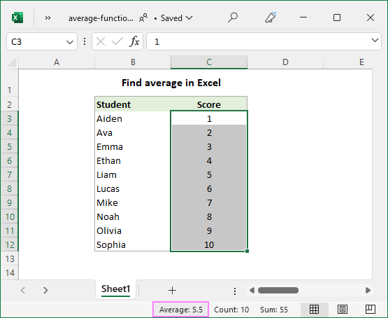
To quickly find an average without a formula, use Excel's status bar:
- Select the cells or ranges you want to average. For non-contiguous selections, use the Ctrl key.
- Look at the status bar at the bottom of the Excel window, which provides the essential information about the currently selected cells. One of the values that Excel calculates automatically is the average.
The result is shown in the image below:
If average is not displayed for your dataset, this article explains possible causes and solutions: Why Excel is not showing sum, average or count in the status bar.
How to calculate average manually
In math, to find the arithmetic mean of a list of numbers, you need to add up all the values, and then divide the sum by how many numbers there are in the list. In Excel, this can be done using the SUM and COUNT functions, respectively:
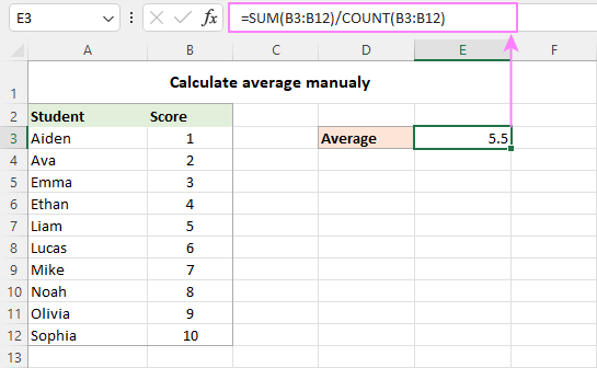
For the range of numbers below, the formula goes as follows:
=SUM(B3:B12)/COUNT(B3:B12)
As you can see, the result of the formula exactly matches the average value in the status bar.
In practice, you will hardly ever need to do a manual average in your worksheets. However, it may be useful to re-check the result of your average formula in case of doubt.
And now, let's take a look at how you can do average in Excel using the functions specially designed for the purpose.
AVERAGE function - calculate an average of numbers
You use the Excel AVERAGE function to get an average of all numbers in the specified cells or ranges.
Where number1, number2, … are numeric values for which you want to find the average. Up to 255 arguments can be included in a single formula. The arguments can be supplied as numbers, references, or named ranges.
AVERAGE is one of the most straightforward and easy-to-use functions in Excel.
To calculate an average of numbers, you can type them directly in a formula or supply the corresponding cell or range references.
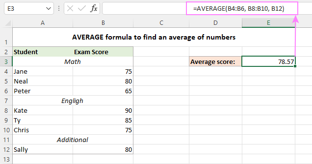
For example, to average 2 ranges and 1 individual cell below, the formula is:
=AVERAGE(B4:B6, B8:B10, B12)
Apart from numbers, the Excel AVERAGE function can find an average of other numeric values such as percentages and times.
Excel AVERAGE formula - usage notes
As you've just seen, using the AVERAGE function in Excel is easy. However, to get a correct result, you need to clearly understand what values are included in the average and what are ignored.
Included:
- Cells with zero values (0)
- Logical values TRUE and FALSE typed directly into the list of arguments. For example, the formula AVERAGE(TRUE, FALSE) returns 0.5, which is the mean of 1 and 0.
Ignored:
- Empty cells
- Text strings
- Cells containing Boolean values TRUE and FALSE
For more information, please see How to use AVERAGE function in Excel.
AVERAGEA function - average all non-blank cells
The Excel AVERAGEA function is similar to AVERAGE in that it calculates the arithmetic mean of the values in its arguments. The difference is that AVERAGEA includes all non-empty cells in a calculation, whether they contain numbers, text, logical values, or empty strings returned by other functions.
Where value1, value2, … are values, arrays, cell references or ranges that you want to average. The first argument is required, others (up to 255) are optional.
Excel AVERAGEA formula - usage notes
As mentioned above, the AVERAGEA function processes different value types such as numbers, text strings and logical values. And here's how they are evaluated:
Included:
- Text values evaluate as 0.
- Zero-length strings ("") evaluate as 0.
- Boolean value TRUE evaluates as 1 and FALSE as 0.
Ignored:
- Empty cells
For example, the below formula returns 1, which is the average of 2 and 0.
=AVERAGEA(2, FALSE)
The following formula returns 1.5, which is the average of 2 and 1.
=AVERAGEA(2, TRUE)
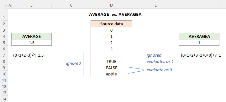
The image below demonstrates the AVERAGE and AVERAGEA formulas applied to the same list of values and different results they return:
AVERAGEIF function - get average with condition
To get the average of all cells in the specified range that meet a certain condition, use the AVERAGEIF function.
The AVERAGEIF function has the following arguments:
- Range (required) - the range of cells to test against a given criteria.
- Criteria (required) - the condition that should be met.
- Average_range (optional) - the cells to average. If omitted, then range is averaged.
The AVERAGEIF function is available in Excel 2007 - Excel 365. In earlier versions, you can build your own AVERAGE IF formula.
And now, let's see how you can use the Excel AVERAGEIF function to average cells based on the condition you specify.
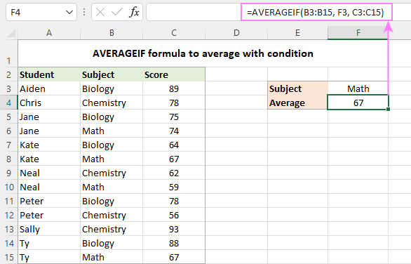
Suppose you have scores for different subjects in C3:C15 and you wish to find an average math score. This can be done with the following formula:
=AVERAGEIF(B3:B15, "math", C3:C15)
Instead of "hardcoding" the condition directly in a formula, you can type it in a separate cell (F3) and refer to that cell in the criteria:
=AVERAGEIF(B3:B15, F3, C3:C15)
For more formula examples, please see Excel AVERAGEIF function.
AVERAGEIFS function - average with multiple criteria
To do average with two or more conditions, use the plural counterpart of AVERAGEIF - the AVERAGEIFS function.
The function has the following syntax:
- Average_range (required) - the range to average.
- Criteria_range (required) - the range to be tested against criteria.
- Criteria (required) - the condition that determines which cells to average. It can be supplied in the form of a number, logical expression, text value, or cell reference.
1 to 127 criteria_range / criteria pairs can be supplied. The first pair is required, subsequent ones are optional.
In essence, you use AVERAGEIFS similarly to AVERAGEIF, except that more than one condition can be tested within a single formula.
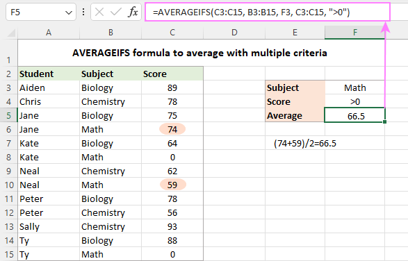
Supposing some students did not take tests in certain subjects and have zero scores. You aim to find an average score in a specific subject ignoring zeros.
To accomplish the task, you build an AVERAGEIFS formula with two criteria:
- Define the range to average (C3:C15).
- Specify the range to check against the 1st condition (B3:B15 - items).
- Express the 1st condition ("math" or F3 - the target item enclosed in quotation marks or reference to the cell containing the item).
- Specify the range to check against the 2nd condition (C3:C15 - scores).
- Express the 2nd condition (">0" - greater than zero).
By assembling the above components together, we get the following formula:
=AVERAGEIFS(C3:C15, B3:B15, "math", C3:C15, ">0")
Or
=AVERAGEIFS(C3:C15, B3:B15, F3, C3:C15, ">0")
The image below makes it clear that only two cells (C6 and C10) meet both conditions, and therefore only these cells are averaged.
For more information, check out Excel AVERAGEIFS function.
AVERAGEIF and AVERAGEIFS formulas - usage notes
Excel AVERAGEIF and AVERAGEIFS functions have much in common, in particular which values they calculate and which ignore:
- In the average range, empty cells, text values, logical values TRUE/FALSE are ignored.
- In criteria, empty cells are treated as zero values.
- The wildcard characters such as question mark (?) and asterisk (*) can be used in criteria for partial match.
- If no cell meets all of the specified criteria, a #DIV0! error occurs.
AVERAGEIF vs. AVERAGEIFS - differences
In terms of functionality, the most essential difference is that AVERAGEIF can only handle one condition while AVERAGEIFS one or more criteria. Also, there are a couple of technical differences related to average_range.
- With AVERAGEIF, average_range is the last and optional argument. In AVERAGEIFS formulas, it is the first and required argument.
- With AVERAGEIF, average_range does not necessarily have to be the same size as range because the actual cells to be averaged are determined by the size of the range argument - the upper left cell of average_range is taken as the starting point, and as many cells are averaged as included in the range argument. AVERAGEIFS requires each criteria_range to be of the same size and shape as average_range, otherwise a #VALUE! error occurs.
AVERAGE IF OR formula in Excel
Since the Excel AVERAGEIFS function always works with the AND logic (all criteria must be TRUE), you will have to construct your own formula to average cells with the OR logic (any single criterion must be TRUE).
Here's the generic formula to average if cell is X or Y.
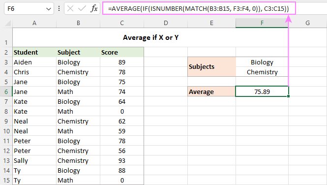
Now, let's see how it works in practice. In the table below, suppose you want to find an average score of two subjects, Biology and Chemistry, which are input in cells F3 and F4. This can be done with the following array formula:
=AVERAGE(IF(ISNUMBER(MATCH(B3:B15, {"biology", "chemistry"}, 0)), C3:C15))
Translated into a human language, the formula says: average cells in C3:C15 if a corresponding cell in B3:B15 is either "Biology" or "Chemistry".
Instead of the hardcoded criteria, you can use a range reference (F3:F4 in our case):
=AVERAGE(IF(ISNUMBER(MATCH(B3:B15, F3:F4, 0)), C3:C15))
For the formula to work correctly, please remember to press Ctrl + Shift + Enter in Excel 2019 and lower. In dynamic array Excel (365 and 2021), a regular Enter hit will suffice:
How this formula works:
For our curious and thoughtful readers who want not only to use a formula but understand what they are doing, here's a detailed explanation of the logic.
At the core of the formula, the IF function determines which values in the source range match any of the specified criteria and passes those values to the AVERAGE function. Here's how:
The MATCH function uses the subject names in B3:B15 as the lookup values and compares each of those values against the lookup array in F3:F4 (our target subjects). The 3rd argument (match_type) is set to 0 to look for exact match:
MATCH(B3:B15, F3:F4, 0)
When a match is found, MATCH returns its relative position in the lookup array, otherwise an #N/A error:
{1;2;1;#N/A;1;#N/A;2;#N/A;1;2;2;1;#N/A}
The ISNUMBER function converts numbers to TRUE and errors to FALSE:
{TRUE;TRUE;TRUE;FALSE;TRUE;FALSE;TRUE;FALSE;TRUE;TRUE;TRUE;TRUE;FALSE}
This array goes to the logical test of IF. In the full form, the logical test should be written like this:
IF(ISNUMBER(MATCH(B3:B15, F3:F4, 0))=TRUE
For the sake of brevity, we omit the =TRUE part because it's implied.
By setting the value_if_true argument to C3:C15, you tell the IF function to replace TRUE's with the actual values from C3:C15:
{89;78;75;FALSE;64;FALSE;62;FALSE;78;56;93;88;FALSE}
This final array is handed over to the AVERAGE function that calculates an arithmetic mean of numbers ignoring logical values.
How to round average in Excel
When calculating an average in Excel, the result is often a number with multiple decimal places. In case you want to display fewer decimal digits or round an average to an integer, use one of the following solutions.
Decrease Decimal option
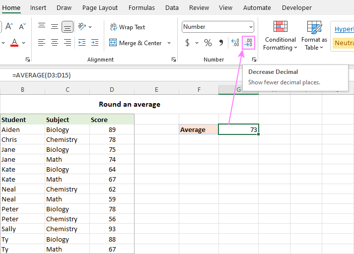
To round only the displayed average without changing the underlying value, the fastest way is to utilize the Decrease Decimal command on the Home tab, in the Number group:
Format Cells dialog box
The number of decimal places can also be specified in the Format Cells dialog box. To have it done, select the formula cell and press Ctrl + 1 to open the Format Cells dialog. Then, switch to the Number tab, and type the number of places you want to show in the Decimal places box.
Like the previous method, this changes only the display format. When referring to the average cell in other formulas, the original non-rounded value will be used in all calculations.

For full details, please see Round numbers by changing cell format.
Round an average with a formula
To round the calculated value itself, wrap your average formula in one of the Excel rounding functions.
In most situations, you'd use the ROUND function that follows the general math rules for rounding. In the 1st argument (number), nest the AVERAGE, AVERAGEIF or AVERAGEIFS function. In the 2nd argument (num_digits), specify the number of decimal places to round the average to.
For example, to round off an average to the nearest integer, the formula is:
=ROUND(AVERAGE(B3:B15), 0)
To round an average to one decimal place, this is the formula to use:
=ROUND(AVERAGE(B3:B15), 1)
To round an average to two decimal places, this one will work:
=ROUND(AVERAGE(B3:B15), 2)

That is how you can do average in Excel. Below there are links to the related tutorials that discuss more specific cases of average, hope you will find them helpful. Thank you for reading!
Practice workbook for download
Calculate average in Excel - examples (.xlsx file)
 by
by
105 comments
please sir i need a formulas basic because i learned first time but i want to learned excel formula
Hello Abbasi,
Hopefully, you will find this tutorial helpful:
Basic Excel formulas & functions with examples
Hi Oscar,
My is Pablo and I would like to ask you about this situation. I have got a column with several values and some of them are zeros. As they are dB measurements this is the array formula I use to get the average: =10*LOG(AVERAGE(10^(C3:C66/10)))
My problem is that I am trying to get with a formula that does not take in account the zeros.
I have tried the next formula but it seems that does not work for my situation: =10*LOG(AVERAGEif(C3:C66,"0",[10^(C3:C66/10)]))
It would be very apprecited if you could give me a hint to solve this problem.
Thank you in advance,
Pablo.
I have multiple columns of dates in excel and am trying to find an average of workdays between the columns. I want Sheet1 to be my trending sheet and Sheet2 to be the data sheet. Column R: Receipt Date, Column S: Processed Date, Column T: Routed Date, Column U: Approved Date. I want the average over the entire columns. Because they are lifecycle dates, some cells may be blank. For example, something may be processed but not yet routed, another item may be processed, routed, and approved, etc.
I need the calculation to show me overall for those items that are both (for example) received and processed, how many days on average it takes to complete processing once the item has been received, etc. (excluding blanks e.g. those items that have neither been received or processed and received but not yet processed)
Right now my calculation is just looking at Column S17:T24 (for troubleshooting and testing) on Sheet 2 and it's "mostly" working and correct but not fully. Once it's fully working and correct I want to move the calculation off to the trending sheet and refer back to the data sheet.
So I have two issues:
1.) I need the calculation to be fully correct.
2.) I need it to be able to refer successfully to another worksheet in the same workbook.
Any help you can provide would be glorious beyond measure!
My current calculation is: {=AVERAGE(IF(NETWORKDAYS(S17:S24+0,T17:T24+0)>0,NETWORKDAYS(S17:S24+0,T17:T24+0),-1))}
I was able to use your help to write a rolling average of my income for the past year, thanks a bunch!
I need help with the following formula. Any suggestions would be appreciated. =AVERAGEIFS(E:E,"=<99.9",M:M,"*A-Shift*")
Dear Svetlana,
Thks for your update.
I learned some shortcuts. I would like to learn the Macro as well. I hope u can suggest better way to learn the Macro.
Kind Regards,
Ram.
Hi Ramaraj,
We have a couple of tutorials on Excel macros. Please check out these ones:
How to insert and run VBA code in Excel - tutorial for beginners
Tutorial with Excel examples about Macros
i need Average
=AVERAGEIF('(Sheet 1)'!A1,'(Sheet 2)'!A1,">1%")
but this formula not put what i do? i need Average different sheets and i want to 0 no count in average.
Like= 0,11,0 =11 Average
in this condition 0 value no coun
Now any input for Max (IF) formula:
=MAX(IF('sheet1'!A:A=J4,'sheet1'!T:T))
In above formula, it consider the Max in column T, by returning name "Truck" in column A. // J4=Truck
Now, if I want to add that dates frame (formula part), how should I go through:
'sheet1'!B:B,">="&P2,'sheet1'!B:B,"<="&P3
P2= Start date
P3= End date
Thanks in advance for your input.
Hello,
Please try the following formula:
=MAXIFS('sheet1'!T:T, 'sheet1'!A:A, J4, 'sheet1'!B:B, ">="&P2, 'sheet1'!B:B, "<="&P3)
Hope it will help you.
Supper thanks finally works :)
an error (,) somewhere in formula :) :) :)
Hello,
All checked and good to go, but still shows #DIV/0! error instead of 2.53 which I calculated manually.
Any other input or any other way to write the formula.
Cheers,
I have a formula which is like this
=AVERAGEIF('sheet1'!A:A,"Truck",'sheet1'!V:V)
which is take the average of all data in column V (sheet1) based on all info related to the Truck in column A.
Now, I want this formula to read the same information but by consider a range of dates in between 1st of October to 15th (I have dates in Column B in the same sheet1).
The formula I created for the second part is like this, but can not merge it to the first part:
'sheet1'!B:B,">="&P2,'sheet1'!B:B,"<="&P3
P2= Start date
P3= End date
Hello,
Please try the following formula:
=AVERAGEIFS('sheet1'V:V,'sheet1'A:A,"Truck",'sheet1'B:B," > ="&P2,'sheet1'B:B," < ="&P3)
Hope it will help you.
Hello and Thanks for your feedback,
It apparently do something, but gave me #DIV/0! error, it should give me a 2.53.
Any input?
Hello,
Please check the following:
1 The ">=" и "<=" conditions in the formula don't contain any spaces.
2 The P2 and P3 cells in your table contain dates.
3 The 'sheet1'!V:V range for calculating an average value is not empty or doesn’t contain text values.
4 The 'sheet1'!A:A and 'sheet1'!B:B ranges with selection criteria are not empty as well.
hi Svetlana
can you please tell me if you can do a similar formula when you need to calculate a nested 'min if' formula and need to ignore the blank cells. This is because when I have blank cells in array of data, the result I get for min if is a blank.
Would really appreciate you help on this
many thanks
Rosh
Can someone help me figure out what is wrong with this function:
{=AVERAGE(IF(CementByRegion!B3:B42,Sheet1!J20,CementByRegion!C3:G42))}
J20="Text" that shows up in column "B". I'm trying to do an average of data in more than one column.
Hello,
I believe this will do :)
=AVERAGEIF(CementByRegion!B3:B42,"="&Sheet1!J20, CementByRegion!C3:G42)
Would you please help me calculate the average of the number of households who treat water per each health volunteer for a duration of 3 months?
=AVERAGE(IF($C$5:$C$310="ACC",$E$5:$E$310,""""))
In this if there is zero value & either cell is blank in E5 to E310 then value should not be count.
"c" "D" "E" "F"
ACC 3200 120 190
ACC 3201
ACC 3400 180 200
ACC 3200
ACC 2989 140 220
ACC 3000
ACC 3050 135 210
Avg of (190,200,220 & 210) showing 82.1
Pls suggest
could you help me to calculate the mean with specific interval in excel.
I have daily data of rainfall for 30 years from that how could i calculate weekly mean easily
Dear Svetlana & Community,
thanks for the great tutorials.
I am trying to average a selection of non-continous columns, all titled "kcal in".
I have set the columns DF2:XA2 as the range, which is the title column. "kcal in" is the crietria and DF4:$XA$435 is the average of all kcal in in the DF4 row. I can drag the formula down to obtain the average for rows DF5 etc.
=AVERAGEIF($DF$2:$XA$2, "kcal in", DF4:$XA$435)
This works well, however, I am trying to exclude any 0 values in row DF4 from the average and I am not sure where to put this criterion.
Many thanks in advance for your help
Found the answer here myself :)
=AVERAGEIFS(DF6:XA6,$DF$2:$XA$2,"kcal in",DF6:XA6,">0")
Adapted from your explanation
Average_range is DF6:XA6 (the row you want to average if both conditions are met);
Criteria_range1 is $DF$2:$XA$2 (the head column, range fixed with dollar sign) and criteria1 is "kcal in"(allowing to average non-continuous columns)
Criteria_range2 is DF6:XA6 (the row you want to average) and criteria2 is ">0". (values of 0 are excluded)
Thanks for the great site, finally my mind can rest :D
Hi , i am trying to find an average based on criteria :
Example 1 : A1 = 3, E1=2 , J1 = 10, My answer will be A1+E1+J1/3 = 5.
Example 2 A1 = 3, E1 = 3, J1 = -, My answer will be A1+E1+J1/3 = 3.
Example 3 A1 = -, E1 = -, J1 = -, My answer should be A1+E1+J1/3 = 0.
Example 1 and 2 is Ok, Where as in example 3 am getting error #DIV/0! instead of this i need 0 in the box.
Thanks in advance
Hi,
please note that empty cells are ignored by AVERAGE function.
Try entering zero (0) in the cells, if you want zero to return.
Hope it helps!
Hi , i am trying to find an average but only based on a certain number of cells in a range. I want to leave the full range in place for the Average formula , but only use part of it based on criteria :
Example : Range A1:M1 carries a forecast of values at start of a Quarter. Three weeks into the Quarter , I then update with Actuals into Cells A1 , B1 , C3 (i.e. i have input 3 cells with Actuals.)
Now i want the average formula for A1:R1 to only use the first 3 cells (which are the Actuals now and the remainder are the Forecast) in my result.
hi, i need to get the average of below data but it seems like im having problem, just one category from type is getting. THANKS SO MUCH IN ADVANCE:)
here's my formula: =AVERAGEIFS(D:D,B:B,"prior20",C:C,"cavite",E:E,{"crtfixed","crtvoice","rbg-crt"})
A B C D
date area ave type
prior20 cavite 10 crtfixed
prior20 cebu 9 crtvoice
prior20 makati 8 rbg-crt
prior20 cavite 7 crtfixed
prior20 cebu 6 crtfixed
prior20 makati 5 crtvoice
prior20 cavite 4 rbg-crt
prior20 cebu 3 crtfixed
beyond luzon 2 crtfixed
prior20 makati 5 crtvoice
prior20 cavite 4 rbg-crt
prior20 cebu 3 crtfixed
Hi Mitch,
try this formula:
=SUM(SUMIFS(D:D,B:B,"prior20",C:C,"cavite",E:E,{"crtfixed","crtvoice","rbg-crt"}))/SUM(COUNTIFS(B:B,"prior20",C:C,"cavite",E:E,{"crtfixed","crtvoice","rbg-crt"}))
I want to auto calculate average of every five cells of a column to another column. I have daily rainfall data for 30 years but I want average of every 5 days of each year.
Hi Jide,
It sounds like you want to calculate a moving average. Please the examples here:
https://www.ablebits.com/office-addins-blog/moving-average-excel/
I have the monthly production but I want to average the documents processed by user per hour
I have following information:
User name Posting Date Time Document no.
1 1/17/2017 13:53:27 xxxxx
1 1/18/2017 9:24:29 xxxxx
2 1/17/2017 15:05:30 xxxxx
3 1/20/2017 12:09:51 xxxxx
4 1/01/2017 12:09:52 xxxxx
5 1/31/2017 08:30:20 xxxxx
hour
have a file with the monthly production and I´m trying to average the invoices process by user per day
Hi Team Ablebits,
can i use AverageIf function for the criteria by font color?
2001 8.5
2002 9
2003 10
2004 18
2005 16
2006 10
2007 11
2008 16.25
2009 14.15
2010 15.5
2011 25
2012 15.5
2013 15.35
2014 13.65
2015 11.86
2016 5.15
i want to calculate the average among the years like 2003-2009 or 2011-2015 etc.
from: 2003 is one cell
to: 2009 is on cell
i m using =AVERAGEIFS(B7:B22,A7:A22,B30&"=>"&"="&B31)
BUT NOT ANSWERING, PLEAE HELP ME IN THIS MATTER.
I want to average multiple cells in a row for each task and then copy down the formula rows below. Each cell has a text value which first needs to be converted to number and then the average calculated. E.g. A1="Start" (which equals 0; B1="Mid Point" (which equals 50) and C1="End" and then Column D1=Average(A1:C1) = ((0+50+100)/3)=50. Formula should work for a range of cells without including the condition (if cell="Start",0,if(cell="Mid Point",50,100))for A1,B1...M1 separately.
I need formula to calculate this data
67 87 86 57 97 86 54 87
determine if the candidate pass PR not if the average score is 55
I am using an AVERAGEIF formula using ranges that have been rounded up and down. When I evaluate my formula the range changes from say 9.0 to 8.999999999 which then means the formula produces a #DIV/0! value.
Can you help with sorting this out please?
Sorry, that should have read AVERAGEIFS
Cheers
Hi, Could you please tell me how can i calculate average excluding blank boxes in excel?
Hi!
By default, the Excel Average function excludes blank cells from an average, though cells with zero values are included.
Hi,
I want to do average of the values using averageif formulae, these values contain 0 also but I want to exclude these Os from the formula.
Please suggest which formula to use.
Hello Avnish,
Use the AVERAGEIFS function and include "is not equal to 0" ("<>"&0) as one of the criteria.
Helo every one.
I'm trying to ge the average for a type of subscription that has 2 names (both are in the same column):
Sub1 and Sub2
(I would like the average for both types together)
However, I also want to restrict to the length of time the subscription has been held ie between two values, say 1 - 3 months.
I think what I'm after is getting the average for OR, and then an AND
Regards
Karon
For relative newcomers or those returning after a long period of non use of Excel, it might have been better to keep it really simple.
I thought it would be straight forward but alas despie reading several internet "help" sources I am no nearer to doing something very simple.
I just have about 650 temperature readings in a column of several thousand.
The range of the 650 is contiguous. I wast the arithmetic average.
"Average(C68:C720)" was the formula I attempted but nothing happens when I press enter.
If it's easy why does this not work, & why if there is "a secret" is it not mentioned?
I have the following formula which works perfectly, however if the lookup value returns no data, I want it to average cells in the previous five rows. Can you help me with a formula to make it work? I have excel 2010
=+IFERROR(VLOOKUP($A6,$A$4:$N$34,9,0),0)
Start Down time End Down Time
11:00 AM 11:05 AM
1:00 PM 1:10 PM
2:30 PM 2:45 PM
Q Write a function in highlighted green cell to get average down time.
I have this formula:
=IFERROR(AVERAGEIFS(Data!G:G,Data!B:B,">=7/1/2016",Data!B:B,"<=7/31/2016",Data!E:E,'Pareto Osmosis'!A33),"-")
I need that this formula change the values of the month that i have in the archive (with respect to column), and, i want to do a little macro to update to the next month. What do i need to do?
=AVERAGEIF(Q2:Q3304, Q2, H2:H3304)
The above formula works for the first of 3304 rows of data. I need to copy the formula down to average the remainder of the scores on each row. I need the middle indicator "Q2" to change based on the row number, but I need the other values to remain the same Q2:Q3304 and H2:H3304.
When I copy the rows down, it wants to change the beginning row for each line.
Ex:
Coping down incorrectly changes it to: =AVERAGEIF(Q3:Q3305, Q3, H3:H3305)--
I need it to be: =AVERAGEIF (Q2:Q3304, Q3, H2:H3304)
Is there a way to do this? Please assist.
Thank you!
I still dont have the answer which l am looking for:
I need a function as if 5 Days average of a certain is 59% and the sixth day l add 30% manually so then its 50% how to bring this in a function
I really like excel, I always try to something new and to learn and this for svetlana Cheusheva...
Hi,
Within Cells A33:A151, I have options of saying either "LISTING" or "DBL END".
In cell N152, my current formula is as follows:
=AVERAGEIF(A33:A151,"LISTING",N33:N151)
This formula works, however, I am having trouble writing the formula so that when a cell within A33:A151 says "DBL END" (as opposed to "LISTING"), Cell N152 still calculates accordingly.
Thanks.
Hi I want include the Zeros between Feb to Aug and exclude the other Zeros for Calculating the Average
Jan Feb Mar Apr May Jun Average
0 505 0 0 346 0 ??
I'm try to create a formula that takes a percentage in four cells per page up to 6 pages. So with a possibility of 24 total entries. that I fill in weekly. Lets say I only have 18 entries that week. So I will like the formula to see that there is only 18 entries and give me the average percentage on those 18 entries not the total 24, the rest will be zero. In the current page the cells are position in (H18,B18,B5,H5) location.
Hi
How can I make the averageifs between two dates work if the average range and the criteria range are in different tabs to the date references?
=AVERAGEIFS('Timeliness SP'!$D$2:$D$10000,'Timeliness SP'!$AM$2:$AM$10000,">="&B66,'Timeliness SP'!$AM$2:$AM$10000,"<"&B67)
This returns Div/0 but if I look at only one date (there are multiple items per date) then it works fine.
Thanks for any help!
80 Fail 92 Pass #DIV/0! #DIV/0!
How get the average and sum this range ?
Please suggest me Pls
Good morning,
We are trying to use the averageifs function over an array of number from C2:O1090 - is this possible as all examples point to a column average only?
Thank you.
Hello Jackie,
Thank you for your question! Until now I haven't realized that all the examples in this tutorial are for a column average, maybe because it's the most typical task.
In fact, you can supply absolutely any range to your Average formula, and even several ranges or individual cells separated by commas. So, the following formula will work just fine:
=AVERAGE(C2:O1090)
Is there any way to use the range in AVERAGEIFS? I have a block of data and need to take the average based on a column criteria and row criteria. Thanks.
A 55
B 60
A
B 20
A
B 30
A 20
AVERAGE
I am working with data spread over 30years and need to find the average for figures which are above 0.5 in the data. I have tried using the averageifs but keeps receiving error message. Attached is a screen shot. Kindly advice how i can proceed.
YEAR MONTH DAY 1 DAY 2 DAY 3 DAY 4 DAY 5 DAY 6
1972 01 0,0 0,0 0,0 0,0 0,0 0,0
1972 02 0,0 0,0 0,0 0,0 0,0 0,0
1972 03 0,0 0,0 0,0 0,0 2,5 0,0
1972 04 0,0 25,2 0,0 0,0 0,0 59,4
1972 05 0,0 0,0 34,0 1,0 0,0 0,0
1972 06 0,0 0,0 0,0 0,0 0,0 0,0
1972 07 0,0 0,0 0,0 0,0 0,0 0,0
1972 08 0,0 0,0 0,3 0,5 0,3 0,0
1972 09 0,0 0,0 0,0 20,3 0,0 0,3
Hello,
I need to find the average but I need the average of the values between two other values, this lasts change with every new range
Thanks,
Svetlana, I have a large data set of over 500 referential urls. The table contains both a count of page views and times spent on the page. I have the following formula that allows me to create a report that gauges interest by keyword in the urls. I need a formula which will filter the following conditions I used in my sumproduct formulat but which will give me an average instead of a sumproduct. Everything I have tried to make this happen has not worked. How can I use what you write above to accomplish this task. Your help would be appreciated. Many Thanks.
=SUMPRODUCT(('RAW DATA'!$A$2:$A$25000=B$336)*
('RAW DATA'!$E$2:$E$25000="micrositeABC")*
(MMULT(0+ISNUMBER(SEARCH(
{"rebate","savings"},
'RAW DATA'!$J$2:$J$25000)
),{1;1})>0),'RAW DATA - PAGE CATEGORIES'!$K$2:$K$25000)
Hello, Thom,
For us to be able to help you better, we need the original math formula you use. Or your workbook with the expected result. You can email the details at support@ablebits.com.
– thanks for dropping by man! I like that you bring in a number of other areas and tie it into creation, I completely agree that this is the mode and task of the church today — to create a forum and median for pattpciiarion [in the Kingdom of God].
Dear Svetlana,
I need to average on a averageifs formula for a range that includes na() and Div/0!
=AVERAGEIFS('SQL Data'!$L$4:$L$65,'SQL Data'!$A$4:$A$65,'sql vs rbct'!$B19,'SQL Data'!$B$4:$B$65,""&'sql vs rbct'!$C19)
This formula above averages between dates and times for the selected date and time range. The data to average is in column l, data in A, times in B.
I have tried the change below but get a value error if I combine the two formulas...
{=AVERAGE(IF(ISNUMBER(Q188:Q194),Q188:Q194))}
Can you help?
Dear Pieter,
For us to be able to assist you better, please send us a small sample table with your data in Excel to support@ablebits.com. Please also include the expected result. Thank you.
range is spelt as rage
Thank you! Fixed.
**spelled
typogrphical error under Excel Average function, second sentence, with bold-face type font