The tutorial shows how to use IF together with the AND function in Excel to check multiple conditions in one formula.
Some things in the world are finite. Others are infinite, and the IF function seems to be one of such things. On our blog, we already have a handful of Excel IF tutorials and still discover new uses every day. Today, we are going to look at how you can use IF together with the AND function to evaluate two or more conditions at the same time.
IF AND statement in Excel
In order to build the IF AND statement, you obviously need to combine the IF and AND functions in one formula. Here's how:
Translated into plain English, the formula reads as follows: IF condition 1 is true AND condition 2 is true, do one thing, otherwise do something else.
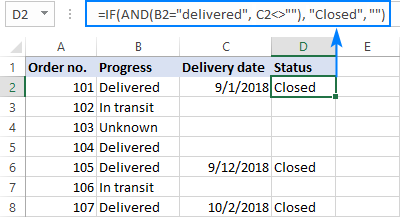
As an example, let's make a formula that checks if B2 is "delivered" and C2 is not empty, and depending on the results, does one of the following:
- If both conditions are TRUE, mark the order as "Closed".
- If either condition is FALSE or both are FALSE, then return an empty string ("").
=IF(AND(B2="delivered", C2<>""), "Closed", "")
The screenshot below shows the IF AND function in Excel:
If you'd like to return some value in case the logical test evaluates to FALSE, supply that value in the value_if_false argument. For example:
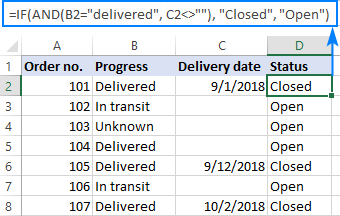
=IF(AND(B2="delivered", C2<>""), "Closed", "Open")
The modified formula outputs "Closed" if column B is "delivered" and C has any date in it (non-blank). In all other cases, it returns "Open":
Note. When using an IF AND formula in Excel to evaluate text conditions, please keep in mind that lowercase and uppercase are treated as the same character. If you are looking for a case-sensitive IF AND formula, wrap one or more arguments of AND into the EXACT function as it is done in the linked example.
Now that you know the syntax of the Excel IF AND statement, let me show you what kind of tasks it can solve.
Excel IF: greater than AND less than
In the previous example, we were testing two conditions in two different cells. But sometimes you may need to run two or more tests on the same cell. A typical example is checking if a cell value is between two numbers. The Excel IF AND function can easily do that too!
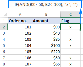
Let's say you have some sales numbers in column B and you are requested to flag the amounts greater than $50 but less than $100. To have it done, insert this formula in C2 and then copy it down the column:
=IF(AND(B2>50, B2<100), "x", "")

If you need to include the boundary values (50 and 100), use the less than or equal to operator (<=) and greater than or equal to (>=) operator:
=IF(AND(B2>=50, B2<=100), "x", "")
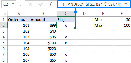
To process some other boundary values without changing the formula, enter the minimum and maximum numbers in two separate cells and refer to those cells in your formula. For the formula to work correctly in all the rows, be sure to use absolute references for the boundary cells ($F$1 and $F$2 in our case):
=IF(AND(B2>=$F$1, B2<=$F$2), "x", "")
By using a similar formula, you can check if a date falls within a specified range.
For example, let's flag dates between 10-Sep-2018 and 30-Sep-2018, inclusive. A small hurdle is that dates cannot be supplied to the logical tests directly. For Excel to understand the dates, they should be enclosed in the DATEVALUE function, like this:
=IF(AND(B2>=DATEVALUE("9/10/2018"), B2<=DATEVALUE("9/30/2018")), "x", "")
Or simply input the From and To dates in two cells ($F$1 and $F$2 in this example) and "pull" them from those cells by using the already familiar IF AND formula:
=IF(AND(B2>=$F$1, B2<=$F$2), "x", "")

For more information, please see Excel IF statement between two numbers or dates.
IF this AND that, then calculate something
Apart from returning predefined values, the Excel IF AND function can also perform different calculations depending on whether the specified conditions are TRUE or FALSE.
To demonstrate the approach, we will be calculating a bonus of 5% for "Closed" sales with the amount greater than or equal to $100.
Assuming the amount is in column B and the order status in column C, the formula goes as follows:
=IF(AND(B2>=100, C2="closed"), B2*10%, 0)

The above formula assigns zero to the rest of the orders (value_if_false = 0). If you are willing to give a small stimulating bonus, say 3%, to orders that do not meet the conditions, include the corresponding equation in the value_if_false argument:
=IF(AND(B2>=100, C2="closed"), B2*10%, B2*3%)

Multiple IF AND statements in Excel
As you may have noticed, we have evaluated only two criteria in all the above examples. But there is nothing that would prevent you from including three and more tests in your IF AND formulas as long as they comply with these general limitations of Excel:
- In Excel 2007 and higher, up to 255 arguments can be used in a formula, with a total formula length not exceeding 8,192 characters.
- In Excel 2003 and lower, no more than 30 arguments are allowed, with a total length not exceeding 1,024 characters.
As an example of multiple AND conditions, please consider these ones:
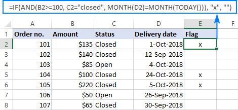
- Amount (B2) should be greater than or equal to $100
- Order status (C2) is "Closed"
- Delivery date (D2) is within the current month
Now, we need an IF AND statement to identify the orders for which all 3 conditions are TRUE. And here it is:
=IF(AND(B2>=100, C2="Closed", MONTH(D2)=MONTH(TODAY())), "x", "")
Given that the 'current month' at the moment of writing was October, the formula delivers the below results:
Nested IF AND statements
When working with large worksheets, chances are that you may be required to check a few sets of different AND criteria at a time. For this, you take a classic Excel nested IF formula and extend its logical tests with AND statements, like this:
To get the general idea, please look at the following example.
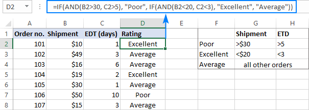
Supposing you want to rate your service based on the shipment cost and estimated time of delivery (ETD):
- Excellent: shipment cost under $20 and ETD under 3 days
- Poor: shipment cost over $30 and ETD over 5 days
- Average: anything in between
To get it done, you write two individual IF AND statements:
IF(AND(B2<20, C2<3), "Excellent", …)
IF(AND(B2>30, C2>5), "Poor", …)
…and nest one into the other:
=IF(AND(B2>30, C2>5), "Poor", IF(AND(B2<20, C2<3), "Excellent", "Average"))
The result will look similar to this:
More formula examples can be found in Excel nested IF AND statements.
Case-sensitive IF AND function in Excel
As mentioned in the beginning of this tutorial, Excel IF AND formulas do not distinguish between uppercase and lowercase characters because the AND function is case-insensitive by nature.
If you are working with case-sensitive data and want to evaluate AND conditions taking into account the text case, do each individual logical test inside the EXACT function and nest those functions into your AND statement:
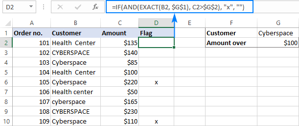
For this example, we are going to flag orders of a specific customer (e.g. the company named Cyberspace) with an amount exceeding a certain number, say $100.
As you can see in the below screenshot, some company names in column B look the same excerpt the characters case, and nevertheless they are different companies, so we have to check the names exactly. The amounts in column C are numbers, and we run a regular "greater than" test for them:
=IF(AND(EXACT(B2, "Cyberspace"), C2>100), "x", "")
To make the formula more flexible, you can input the target customer name and amount in two separate cells and refer to those cells. Just remember to lock the cell references with $ sign ($G$1 and $G$2 in our case) so they won't change when you copy the formula to other rows:
=IF(AND(EXACT(B2, $G$1), C2>$G$2), "x", "")
Now, you can type any name and amount in the referenced cells, and the formula will flag the corresponding orders in your table:
IF OR AND formula in Excel
In Excel IF formulas, you are not limited to using only one logical function. To check various combinations of multiple conditions, you are free to combine the IF, AND, OR and other functions to run the required logical tests. Here is an example of IF AND OR formula that tests a couple of OR conditions within AND. And now, I will show you how you can do two or more AND tests within the OR function.
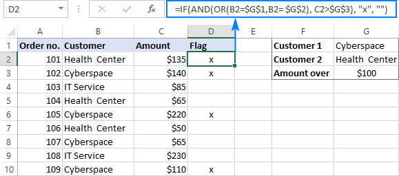
Supposing, you wish to mark the orders of two customers with an amount greater than a certain number, say $100.
In the Excel language, our conditions are expressed in this way:
OR(AND(Customer1, Amount>100), AND(Customer2, Amount>100)
Assuming the customer names are in column B, amounts in column C, the 2 target names are in G1 and G2, and the target amount is in G3, you use this formula to mark the corresponding orders with "x":
=IF(OR(AND(B2=$G$1, C2>$G$3), AND(B2=$G$2, C2>$G$3)), "x", "")
The same results can be achieved with a more compact syntax:
=IF(AND(OR(B2=$G$1,B2= $G$2), C2>$G$3), "x", "")
Not sure you totally understand the formula's logic? More information can be found in Excel IF with multiple AND/OR conditions.
That's how you use the IF and AND functions together in Excel. Thank you for reading and see you next week!
Practice workbook
IF AND Excel – formula examples (.xlsx file)
 by
by
309 comments
Hello,
I need a formula that will tell me:
If A1 is specific "business unit #", then a2 will pull "name of said business unit" from worksheet2.
The data for a2 is on a separate worksheet.
Thank you,
Pam
Hi! The answer to your question can be found in this article: Vlookup from another sheet.
Hi, I am trying to create a formula that says if B2 is gloss and B3 is 5 then result is .45 also if B2 is matte and B3 is 5 then output is .61.
I need to do this for 3, 5, and 10 and also an argument for a third variable searching for "digital" and giving a different output for that.
Something similar to this:
=IF(ISNUMBER(SEARCH("SCUFF",B2)),".325",IF(ISNUMBER(SEARCH("SOFT",B2)),".34",IF(ISNUMBER(SEARCH("MATTE",B2)),".119",IF(ISNUMBER(SEARCH("GLOSS",B2)),".109",""))))
But I need to output a different value of .70 if the word "digital" is included.
Thanks in advance!
Robert
Can we have 36 IF and AND condition in one cell? [for e.g. =IF(AND(D6="Extreme", E6="Minimal"), "Moderate"), IF(AND(D6="Extreme", E6="Minor"), "Significant"), IF(AND(D6="Extreme",E6="Moderate"),"High"), IF(AND(D6="Extreme",E6="Major"),"Extreme")].. This is just 4, I have another 34 such conditions to add... I am not sure where is the mistake .. Can you please help
Hi! In your case, for a large number of conditions, I recommend using the IFS function. Look for the example formulas here: Excel IFS function instead of multiple IF.
These guidelines may also be helpful: Excel Nested IF statements - examples, best practices and alternatives. I hope it’ll be helpful.
Hey
I'm trying to achieve the following:
A2 has a conditional list full of customers
B2 has a conditional list of yes or no option for certain manufacture option 1
C2 has a conditional list of yes or no option for certain manufacture option 2
D2 will show an output of which workplan is needed to be selected
I have tried the following IF statement, to no use:
=IF(AND(A2="XX"),"X1 Workplan",IF(AND(B2="Yes"),"X2 Workplan",IF(AND(C2="Yes"),"X3 Workplan")))
If anyone can help, that would be great!
Hi Mark!
It is very difficult to help you, as it is impossible to guess what goal you want to achieve. Note to your formula: you don't need to use the AND function if there is only one condition.
Is there a way to make the below work?
=IF(And(FN$2=$I$6:$I$101), FN$1, ""), IF(AND(FN$4=$I$6:$I$101), FN$1, "")
Hi! IF function doesn't work with arrays. If I understand your task correctly, the following formula should work for you:
=IF(PRODUCT(--(FN$2=$I$6:$I$101)), FN$1, "")
Need some assistance in writing an excel formula for the below. I tried many of the suggestions without success.
If a cell has a value with either 1 or 2, populate PM; if the same cell has value 3 or 4, populate ME and if same cell has value 5, populate EE.
I know it's a greater than on less than, but my formula is still not working, even the nested is not working.
PM - score achieved 1-2 points
ME - score achieved 3-4 points
EE - score achieved 5 points
Values 1, 2, 3, 4 or 5 will be in the same cell.
Thank you for your assistance.
Hello Marcia!
You can find the answer to your question in this article: Excel Nested IF statement: examples, best practices and alternatives. Here are some variations of the formula:
=IF(A1>=5,"EE",IF(A1>=3,"ME","PM"))
=IFERROR(IFS(A1>=5,"EE",A1>=3,"ME",A1>=1,"PM"),"")
=IFERROR(CHOOSE(A1,"PM","PM","ME","ME","EE"),"")
I did try the nested if statement but it didn't work...maybe an error on my part.
Thank you so much for responding. I will try these.
The 1st option worked. Apparently the cell I was inputted the formula was corrupted...something within the cell was throwing an error. I deleted the rows and re-entered the formula and it worked. Thank you!!!
Hello, Can you please help with this formula =IF(AND(H3="Female",I3="Married",D3<=50,K3="Cat A"),Pricing!E2),IF(AND(H3="Female",I3="Married",D3<=50,K3="Cat B"),Pricing!E9) insurance premium does not change when it changes to "Cat B". Not sure why? Appreciate your help
Hi! Your formula contains a syntax error. Look for the example formulas here: Nested IF in Excel – formula with multiple conditions. For example:
=IF(AND(H3="Female",I3="Married",D3<=50,K3="Cat A"),Pricing!E2, IF(AND(H3="Female",I3="Married",D3<=50,K3="Cat B"),Pricing!E9))
I'm trying to track the progress of a job. I have 4 columns; each have a date entered when the task is completed. I have a 5th column reporting the status, but I can't get past the first status. When the first date is entered, it says "ready". But when the second, third, and fourth dates are entered, it doesn't change to "in progress", "finished", "complete". Is it possible to create this function?
Hello Karie!
If I understand your task correctly, this article may be helpful: Nested IF in Excel – formula with multiple conditions. The formula might look something like the following:
=IF(D1<>"","complete",IF(C1<>"","Finished",IF(B1<>"","in progress",IF(A1<>"","ready",""))))
Thank you!! This is exactly what I needed!
Hi,
I am racking my brain on what is wrong with this and I have tried several variations. I am trying to see if my value on my main sheet matches the 2 out of 3 values on three other sheets.
A2 is the cell I am checking and if present in 2/3 sheets I want it to be reported.
VF and SCI and 2 different sheets and the A2 value can be in either or of these but needs to be in one of them
CR is a submission sheet and A2 100% needs to be here.
I have tried the following:
=if(and(or(A2 ='VF'!A$2:A209,A2='CR'!E$2:E1209, A2='SCI'!A$2:A209)),A2, "Check ERROR") - states its correct but I know it should show up as an error
=if(and(or(A2='CR'!E$2:E1224), A2 ='VF!A$2:A224, A2='SCI'!A$2:A224),A2, "Check ERROR") - states error
=if(and(A7 ='Valley Fever Case Information'!A$2:A214,A7='Case Reports'!E$2:E1214),A7, if(and(A7='Salmonella Case Information'!A$2:A214,A7='Case Reports'!E$2:E1214),A7, "Check ERROR")) - states error.
Any help would be great
=
Hi! If I understand your task correctly, the following formula should work for you:
=IF(ISNUMBER(MATCH(2,(A2=vf!A$2:A209)+(A2=cr!E$2:E209)+(A2=sci!A$2:A209),0)),A2,"")
Use the MATCH function to find the position where the desired value is written on the 2 worksheets.
I hope it’ll be helpful.
I am placing/writing a formula in cell C1
In A1 - Its EXPIRY DATE
In B1 - Its RENEWAL DATE
=IF(TODAY()>=B1,"SEND RENEW REMINDER","WAIT")
The above formula is working.
Now, I want to apply one more condition in same cell C1 - That if A1 is less than TODAY's date, the result should be "PENDING" and if I write manually (CANCELLED) in A1, the result should be "CANCELLED". Something like =IF(TODAY()<A1,"PENDING") =IF(A1=CANCELLED,"CANCELLED")
I am finding difficulty to apply the second condition merging with first condition in the same cell.
Please help me out.
Hi! To write multiple conditions in an IF formula, you can use this guide: Nested IF in Excel – formula with multiple conditions. For example:
=IF(TODAY()<A1,"PENDING", IF(TODAY()>=B1,"SEND RENEW REMINDER","WAIT"))
What is Wrong with this formula, it is giving ERROR:
IF(AND(N15="ACRE",P15="BIGHA”),M15*3.02500,IF(AND(N15="ACRE",P15="KATHA”),M15*60.50000,IF(AND(N15="KATHA",P15="ACRE”),M15*0.01653,IF(AND(N15="BIGHA",P15="ACRE”),M15*0.33058,IF(AND(N15="KATHA",P15="SQ.FT.”),M15*720.00003,IF(AND(N15="KATHA",P15="CHHATAK”),M15*16.00000,IF(AND(N15="CHHATAK",P15="KATHA”),M15*0.06250,IF(AND(N15="KATHA",P15="DECIMAL”),M15*1.65289256,IF(AND(N15="DECIMAL",P15="KATHA”),M15*0.60500,IF(AND(N15="ACRE",P15="SQ.FT.”,M15*43560,IF(AND(N15="SQ.FT.",P15="ACRE”,M1/43560)))))))))))
Hi! Check the quotation marks in your formula. Use " instead of ”
Looking for some guidance please..
I have 3 IF formulas - all functioning as i need them to in separate cells. however i am struggling to nest them. For context i am creating a diary that will flag up dates for various conditions.
the 3 formulas are as follows :
1- =IF(H2>=TODAY()+8,"OVER 7 DAYS", "")
2- =IF(AND(H2>=TODAY()+1,H2<=TODAY()+7),"WITHIN 7 DAYS","")
3- =IF(H2=TODAY()+8),"OVER 7 DAYS", IF(AND(H2>=TODAY()+1),(H2<=TODAY()+7)),"WITHIN 7 DAYS", IF((H2=TODAY()+8),"OVER A WEEK", (H2>=TODAY()+1 & H2<=TODAY()+7), "WITHIN 7 DAYS" , (H2<=TODAY()), "TODAY / OVERDUE", "")
Thanks in advance for any guidance on why i'm not getting anywhere !
The error is too many functions is there a way around this ?
Hello! If you have too many conditions in your formula, I recommend using the IFS function instead of the nested IF. Based on the information given, the formula could be as follows:
=IFS(H2>=TODAY()+8, "OVER 7 DAYS", AND(H2>=TODAY()+1,H2<=TODAY()+7), "WITHIN 7 DAYS", H2=TODAY()+8,"OVER 7 DAYS", H2=TODAY()+8,"OVER A WEEK", H2<=TODAY(), "TODAY / OVERDUE")
You can find the examples and detailed instructions here: The new Excel IFS function instead of multiple IF.
=IF(AND(C5>120,160<D5<200,1.59<E5120,160<D5<200,1.59<E5120,160<D5<200,1.59<E5120,160<D5<200,1.59<E5120,201<D5<280,4.8<E5120,201<D5<280,4.8<E5120,201<D5<280,4.8<E5120,201<D5<280,4.8<E5120,D5>280,15.6<E5120,D5>280,15.6<E5120,D5>280,15.6<E5120,D5>280,15.6<E5<35.4,F5="Boulder"),1000,""))))))))))))
What is wrong with this that it cant give me an out put?
Hi! Your formula contained errors. Leave only one parenthesis at the end of the formula.
Strength(mg) Quantity
250mg 1 tablet
500mg 2 tablets
750mg 3 tablets
1000mg 4 tablets
1250mg 5 tablets
1500mg 6 tablets
1750mg 7 tablets
2000mg 8 tablets
2250mg 9 tablets
2500mg 10 tablets
How do i set a cell that when i enter any mg in D26, it should tell me the value of tablets depends in the tablet. for eg: 251mg, it must input 2 tablets and 249mg, it must input 1 tablet.
Thank you.
Hi! To find the first value in the table that is greater than the criterion, use the XLOOKUP function
=XLOOKUP(D1,A1:A10,B1:B10,,1)
You can also use the INDEX MATCH functions:
=INDEX(B1:B10, MATCH(TRUE, INDEX(A1:A10 >= D1, 0), ))
Note that column A must contain numbers, not text. That is, 250, not 250mg.
I am trying to check if a state and email address are the same across two different data sets. Eg email @email.com and Arizona are the matching in both lists. Any help is welcome
Hi! Try to use the recommendations described in this article: Compare two columns for matches and differences. If this is not what you wanted, please describe the problem in more detail.
I HAVE TYPED THIS WHOLE FORMULA BUT ITS OVER LIMIT FORMULAS...HOW CAN I USE THIS LENGTHY FORMULA
=IF(AND(F2=15,F2=25,K2="AJ"),F2*20,
IF(AND(F2=15,F2=25,K229="ANIL"),F2*20,
IF(AND(F2=15,K2="AR"),F2*30,
IF(AND(F2=15,K2="BH"),F2*25,
IF(AND(F2=15,F2=25,K2="BHAVANI"),F2*25,
IF(AND(F2=15,F2=25,K2="BK"),F2*20
IF(AND(F2=25,K2="BR"),F2*18,
IF(AND(F2=15,F2=25,K2="DATAR"),F2*25,
IF(AND(F2=15,F2=25,K2="ECO"),F2*30,
IF(AND(F2=15,F2=25,K2="GHN"),F2*25,
IF(AND(F2=15,F2=25,K2="HG"),F2*25,
IF(AND(F2=25,K2="HL"),F2*30,
IF(AND(F2=15,K2="KS"),F2*20,
IF(AND(F2=15,K2="LAXIT"),F2*25,
IF(AND(F2=15,F2=25,K2="MAHESH"),F2*50,
IF(AND(F2=25,K2="MEHUL"),F2*25,
IF(AND(F2=15,F2=25,K2="MI"),F2*25,
IF(AND(F2=15,F2=25,K2="MIRA"),F2*25,
IF(AND(F2=15,F2=25,K2="MK"),F2*25,
IF(AND(F2=15,F2=25,K2="ND"),"300",
IF(AND(F2=15,F2=25,K2="PAN"),F2*25,
IF(AND(F2=15,F2=25,K2="PG"),F2*23,
IF(AND(F2=15,F2=25,K2="PP"),F2*25,
IF(AND(F2=15,K2="PRADIP"),F2*20,
IF(AND(F2=15,K2="PURU"),F2*30,
IF(AND(F2=15,K2="RAJ303"),F2*30,
IF(AND(F2=15,K2="RP"),F2*25,
IF(AND(F2=15,F2=25,K2="SG"),F2*25,
IF(AND(F2=15,F2=25,K2="SJ"),"500",
IF(AND(F2=15,K2="VINIT"),"500",
IF(AND(F2=15,K2="SNK"),F2*30,
IF(AND(F2=15,F2=25,K2="SP"),"500",
IF(AND(F2=15,F2=25,K2="SS3",
IF(AND(F2=15,F2=25,K2="SUN"),F2*23,
IF(AND(F2=15,F2=25,K2="VD"),F2*70,
IF(AND(F2=15,F2=25,K2="VI"),F2*22,
IF(AND(F2=15,F2=25,K2="VINIT"),F2*21,
IF(AND(F2=15,F2=25,K2="VISHAL",
IF(AND(F2=15,K2="ZD"),F2*20)))))))))))))
Hi! Try to follow the recommendations from this article: Use the new Excel IFS function instead of nested IF.
Hello! I'm a bit stuck after trying multiple IF AND functions to return a single value in a cell. The following is what I have so far:
=IF(AND(ISNUMBER(SEARCH("ACCOUNT 1",[@[Account name]])), SEARCH("Nonbrand",[@Category])),"Nonbrand", IF(AND(ISNUMBER(SEARCH("ACCOUNT 1",[@[Account name]])), SEARCH("Branded",[@Category])),"Branded", IF(ISNUMBER(SEARCH("ACCOUNT 2",[@[Account name]])),"PLA","Other")))
Currently the function returns "Nonbrand" but not "Branded" or "PLA" which are all of my desired values based on the criteria; the latter two are returned as #VALUE!
Hopefully this is enough information, but please let me know if I should add more context. Thank you for your help!
Hi! I can't validate a calculation that contains unique references to your data that I do not have. The #VALUE! error can occur in SEARCH("Nonbrand",[@Category]) SEARCH("Branded",[@Category]) because you are not using ISNUMBER.
Hi please need your help on this scenario If cell less than 50 is equal to zero and If cell greater than 50 then add the over whats the formula? I tried this formula =IF(AND(A150,50-A1))
Hoping for your help on this formula.. Thank you in advance
Hi! The following tutorial should help: IF formula for numbers.
I need help with a formula please. I have amounts in columnA1, if a1 is under 100 I want the amount in b1, if not I want it in c1
Hi! The answer to your question can be found in this article: IF function in Excel: formula examples for text, numbers, dates, blanks. IF(A1<100,B1,C1)
I have three shifts (1,2,3) on the drop down menu in column G. If it is the first shift it should show the results in column A from column B, if it is the second shift it should show the results in column A from column C, if it is the third shift it should show the result in column A from column D. I need the formula. Thank you
Hi! If I understand your task correctly, you can see examples of formulas for your task in this article: Excel Nested IF statement: examples, best practices and alternatives. For example:
=IF(G1=1,B1,IF(G1=2,C1,IF(G1=3,D1),""))
or
=IFS(G1=1,B1,G1=2,C1,G1=3,D1)
or
=CHOOSE(G1,B1,C1,D1)