 by
by In this tutorial, you will find a number of formula examples that demonstrate the most efficient uses of INDEX in Excel.
Of all Excel functions whose power is often underestimated and underutilized, INDEX would definitely rank somewhere in the top 10. In the meantime, this function is smart, supple and versatile.
So, what is the INDEX function in Excel? Essentially, an INDEX formula returns a cell reference from within a given array or range. In other words, you use INDEX when you know (or can calculate) the position of an element in a range and you want to get the actual value of that element.
This may sound a bit trivial, but once you realize the real potential of the INDEX function, it could make crucial changes to the way you calculate, analyze and present data in your worksheets.
Excel INDEX function - syntax and basic uses
There are two versions of the INDEX function in Excel - array form and reference form. Both forms can be used in all versions of Microsoft Excel 365 - 2016.
INDEX array form
The INDEX array form returns the value of a certain element in a range or array based on the row and column numbers you specify.
array- is a range of cells, named range, or table.row_num- is the row number in the array from which to return a value. Ifrow_numis omitted,column_numis required.column_num- is the column number from which to return a value. If column_num is omitted, row_num is required.
For example, the formula =INDEX(A1:D6, 4, 3) returns the value at the intersection of the 4th row and 3rd column in range A1:D6, which is the value in cell C4.
To get an idea of how the INDEX formula works on real data, please have a look at the following example:
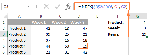
Instead of entering the row and column numbers in the formula, you can supply the cell references to get a more universal formula:
=INDEX($B$2:$D$6, G2, G1)
So, this INDEX formula returns the number of items exactly at the intersection of the product number specified in G2 (row_num) and week number entered in cell G1 (column_num).
Tip. The use of absolute references $B$2:$D$6 instead of relative references B2:D6 in the array argument makes it easier to copy the formula to other cells. Alternatively, you can convert a range to a table (Ctrl + T) and refer to it by the table name.
INDEX array form - things to remember
- If the array argument consists of only one row or column, you may or may not specify the corresponding
row_numorcolumn_numargument. - If the array argument includes more than one row and
row_numis omitted or set to 0, the INDEX function returns an array of the entire column. Similarly, if array includes more than one column and thecolumn_numargument is omitted or set to 0, the INDEX formula returns the entire row. Here's a formula example that demonstrates this behavior. - The
row_numandcolumn_numarguments must refer to a cell within array; otherwise, the INDEX formula will return the#REF!error.
INDEX reference form
The reference form of the Excel INDEX function returns the cell reference at the intersection of the specified row and column.
reference- is one or several ranges.If you are entering more than one range, separate the ranges by commas and enclose the reference argument in parentheses, for example(A1:B5, D1:F5).If each range in reference contains only one row or column, the corresponding
row_numorcolumn_numargument is optional.row_num- the row number in the range from which to return a cell reference, it's similar to the array form.column_num- the column number from which to return a cell reference, also works similarly to the array form.area_num- an optional parameter that specifies which range from the reference argument to use. If omitted, the INDEX formula will return the result for the first range listed in reference.
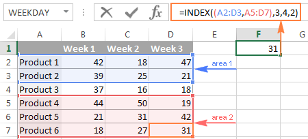
For example, the formula
=INDEX((A2:D3, A5:D7), 3, 4, 2) returns the value of cell D7, which is at the intersection of the 3rd row and 4th column in the second area A5:D7.
INDEX reference form - things to remember
- If the
row_numorcolumn_numargument is set to zero (0), an INDEX formula returns the reference for the entire column or row, respectively. - If both
row_numandcolumn_numare omitted, the INDEX function returns the area specified in thearea_numargument. - All of the _num arguments (
row_num,column_numandarea_num) must refer to a cell within reference; otherwise, the INDEX formula will return the#REF!error.
Both of the INDEX formulas we've discussed so far are very simple and only illustrate the concept. Your real formulas are likely to be far more complex than that, so let's explore a few most efficient uses of INDEX in Excel.
How to use INDEX function in Excel - formula examples
Perhaps there aren't many practical uses of Excel INDEX by itself, but in combination with other functions such as MATCH or COUNTA, it can make very powerful formulas.
Source data
All of our INDEX formulas (except for the last one), we will use the below data. For convenience purposes, it is organized in a table named SourceData.
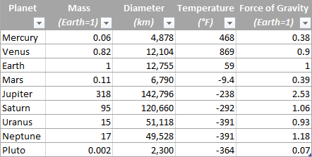
The use of tables or named ranges can make formulas a bit longer, but it also makes them significantly more flexible and better readable. To adjust any INDEX formula for your worksheets, you need only to modify a single name, and this fully makes up for a longer formula length.
Of course, nothing prevents you from using usual ranges if you want to. In this case, you simply replace the table name SourceData with the appropriate range reference.
1. Getting the Nth item from the list
This is the basic use of the INDEX function and a simplest formula to make. To fetch a certain item from the list, you just write =INDEX(range, n) where range is a range of cells or a named range, and n is the position of the item you want to get.
When working with Excel tables, you can select the column using the mouse and Excel will pull the column's name along with the table's name in the formula:
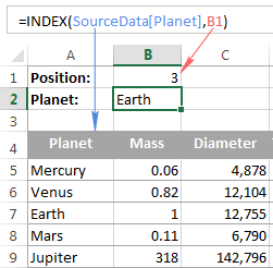
To get a value of the cell at the intersection of a given row and column, you use the same approach with the only difference that you specify both - the row number and the column number. In fact, you already saw such a formula in action when we discussed INDEX array form.
And here's one more example. In our sample table, to find the 2nd biggest planet in the Solar system, you sort the table by the Diameter column, and use the following INDEX formula:
=INDEX(SourceData, 2, 3)
Arrayis the table name, or a range reference, SourceData in this example.Row_numis 2 because you are looking for the second item in the list, which is in the 2ndColumn_numis 3 because Diameter is the 3rd column in the table.
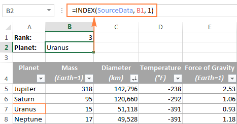
If you want to return the planet's name rather than diameter, change column_num to 1. And naturally, you can use a cell reference in the row_num and/or column_num arguments to make your formula more versatile, as demonstrated in the screenshot below:
2. Getting all values in a row or column
Apart from retrieving a single cell, the INDEX function is able to return an array of values from the entire row or column. To get all values from a certain column, you have to omit the row_num argument or set it to 0. Likewise, to get the entire row, you pass empty value or 0 in column_num.
Such INDEX formulas can hardly be used on their own, because Excel is unable to fit the array of values returned by the formula in a single cell, and you would get the #VALUE! error instead. However, if you use INDEX in conjunction with other functions, such as SUM or AVERAGE, you will get awesome results.
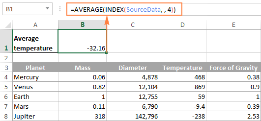
For example, you could use the following formula to calculate the average planet temperature in the Solar system:
=AVERAGE(INDEX(SourceData, , 4)) In the above formula, the column_num argument is 4 because Temperature in the 4th column in our table. The row_num parameter is omitted.
In a similar manner, you can find the minimum and maximum temperatures:
=MAX(INDEX(SourceData, , 4)) =MIN(INDEX(SourceData, , 4))
And calculate the total planet mass (Mass is the 2nd column in the table):
=SUM(INDEX(SourceData, , 2))
From practical viewpoint, the INDEX function in the above formula is superfluous. You can simply write =AVERAGE(range) or =SUM(range) and get the same results.
When working with real data, this feature may prove helpful as part of more complex formulas you use for data analysis.
3. Using INDEX with other functions (SUM, AVERAGE, MAX, MIN)
From the previous examples, you might be under an impression that an INDEX formula returns values, but the reality is that it returns a reference to the cell containing the value. And this example demonstrates the true nature of the Excel INDEX function.
Since the result of an INDEX formula is a reference, we can use it within other functions to make a dynamic range. Sounds confusing? The following formula will make everything clear.
Suppose you have a formula =AVERAGE(A1:A10) that returns an average of the values in cells A1:A10. Instead of writing the range directly in the formula, you can replace either A1 or A10, or both, with INDEX functions, like this:
=AVERAGE(A1 : INDEX(A1:A20,10))
Both of the above formulas will deliver the same result because the INDEX function also returns a reference to cell A10 (row_num is set to 10, column_num omitted). The difference is that the range is the AVERAGE / INDEX formula is dynamic, and once you change the row_num argument in INDEX, the range processed by the AVERAGE function will change and the formula will return a different result.
Apparently, the INDEX formula's route appears overly complicated, but it does have practical applications, as demonstrated in the following examples.
Example 1. Calculate average of the top N items in the list
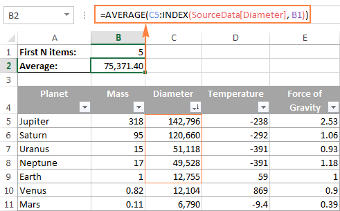
Let's say you want to know the average diameter of the N biggest planets in our system. So, you sort the table by Diameter column from largest to smallest, and use the following Average / Index formula:
=AVERAGE(C5 : INDEX(SourceData[Diameter], B1))
Example 2. Sum items between the specified two items
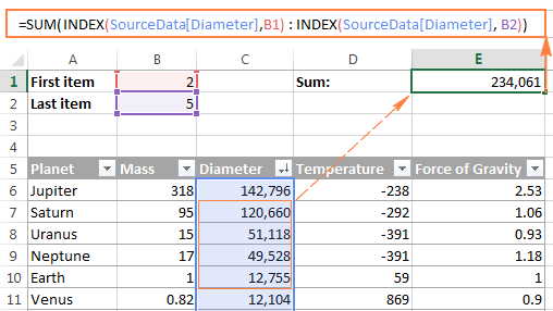
In case you want to define the upper-bound and lower-bound items in your formula, you just need to employ two INDEX functions to return the first and the last item you want.
For example, the following formula returns the sum of values in the Diameter column between the two items specified in cells B1 and B2:
=SUM(INDEX(SourceData[Diameter], B1) : INDEX(SourceData[Diameter], B2))
4. INDEX formula to create dynamic ranges and drop-down lists
As it often happens, when you start organizing data in a worksheet, you may not know how many entries you will eventually have. It's not the case with our planets table, which seems to be complete, but who knows...
Anyway, if you have a changing number of items in a given column, say from A1 to An, you may want to create a dynamic named range that includes all cells with data. At that, you want the range to adjust automatically as you add new items or delete some of the existing ones. For example, if you currently have 10 items, your named range is A1:A10. If you add a new entry, the named range automatically expands to A1:A11, and if you change your mind and delete that newly added data, the range automatically reverts to A1:A10.
The main advantage of this approach is that you do not have to constantly update all formulas in your workbook to ensure they refer to correct ranges.
One way to define a dynamic range is using Excel OFFSET function:
=OFFSET(Sheet_Name!$A$1, 0, 0, COUNTA(Sheet_Name!$A:$A), 1)
Another possible solution is to use Excel INDEX together with COUNTA:
=Sheet_Name!$A$1:INDEX(Sheet_Name!$A:$A, COUNTA(Sheet_Name!$A:$A))
In both formulas, A1 is the cell containing the first item of the list and the dynamic range produced by both formulas will be identical.
The difference is in the approaches. While the OFFSET function moves from the starting point by a certain number of rows and/or columns, INDEX finds a cell at the intersection of a particular row and column. The COUNTA function, used in both formulas, gets the number of non-empty cells in the column of interest.
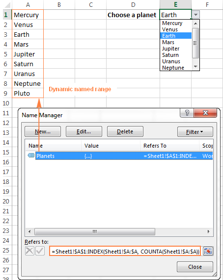
In this example, there are 9 non-blank cells in column A, so COUNTA returns 9. Consequently, INDEX returns $A$9, which is the last used cell in column A (usually INDEX returns a value, but in this formula, the reference operator (:) forces it to return a reference). And because $A$1 is our starting point, the final result of the formula is the range $A$1:$A$9.
The following screenshot demonstrates how you can use such Index formula to create a dynamic drop-down list.
Tip. The easiest way to create an expandable dynamic data validation list is dropdown from a table. In this case, you won't need any complex formulas since Excel tables are dynamic ranges per se.
You can also use the INDEX function to create dependent drop-down lists and the following tutorial explains the steps: Making a cascading drop-down list in Excel.
5. Powerful Vlookups with INDEX / MATCH
Performing vertical lookups - this is where the INDEX function truly shines. If you have ever tried using Excel VLOOKUP function, you are well aware of its numerous limitations, such as inability to pull values from columns to the left of the lookup column or 255 chars limit for a lookup value.
The INDEX / MATCH liaison is superior to VLOOKUP in many respects:
- No problems with left vlookups.
- No limit to the lookup value size.
- No sorting is required (VLOOKUP with approximate match does require sorting the lookup column in ascending order).
- You are free to insert and remove columns in a table without updating every associated formula.
- And the last but not the least, INDEX / MATCH does not slow down your Excel like multiple Vlookups do.
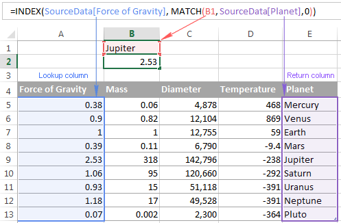
You use INDEX / MATCH in the following way:
For example, if we flip our source table so that Planet Name becomes the right-most column, the INDEX / MATCH formula still fetches a matching value from the left-hand column without a hitch.
For more tips and formula example, please see the Excel INDEX / MATCH tutorial.
6. Excel INDEX formula to get 1 range from a list of ranges
Another smart and powerful use of the INDEX function in Excel is the ability to get one range from a list of ranges.
Suppose, you have several lists with a different number of items in each. Believe me or not, you can calculate the average or sum the values in any selected range with a single formula.
First off, you create a named range for each list; let it be PlanetsD and MoonsD in this example:
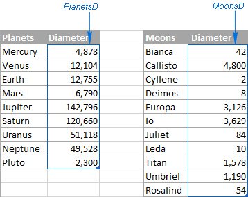
I hope the above image explains the reasoning behind the ranges' names : ) BTW, the Moons table is far from complete, there are 176 known natural moons in our Solar System, Jupiter alone has 63 currently, and counting. For this example, I picked random 11, well… maybe not quite random - moons with the most beautiful names : )
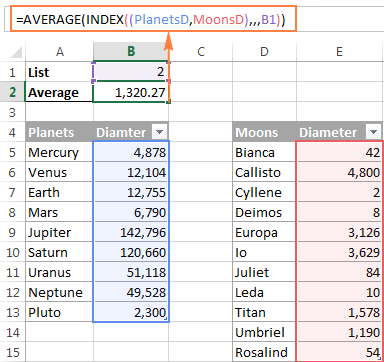
Please excuse the digression, back to our INDEX formula. Assuming that PlanetsD is your range 1 and MoonsD is range 2, and cell B1 is where you put the range number, you can use the following Index formula to calculate the average of values in the selected named range:
=AVERAGE(INDEX((PlanetsD, MoonsD), , , B1))
Please pay attention that now we are using the Reference form of the INDEX function, and the number in the last argument (area_num) tells the formula which range to pick.
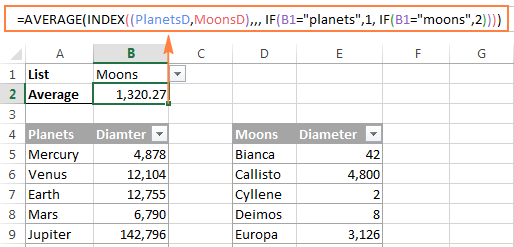
In the screenshot below, area_num (cell B1) is set to 2, so the formula calculates the average diameter of Moons because the range MoonsD comes 2nd in the reference argument.
If you work with multiple lists and don't want to bother remembering the associated numbers, you can employ a nested IF function to do this for you:
=AVERAGE(INDEX((PlanetsD, MoonsD), , , IF(B1="planets", 1, IF(B1="moons", 2))))
In the IF function, you use some simple and easy-to-remember list names that you want your users to type in cell B1 instead of numbers. Please keep this in mind, for the formula to work correctly, the text in B1 should be exactly the same (case-insensitive) as in the IF's parameters, otherwise your Index formula will throw the #VALUE error.
To make the formula even more user-friendly, you can use Data Validation to create a drop-down list with predefined names to prevent spelling errors and misprints:
Finally, to make your INDEX formula absolutely perfect, you can enclose it in the IFERROR function that will prompt the user to choose an item from the drop-down list if no selection has been made yet:
=IFERROR(AVERAGE(INDEX((PlanetsD, MoonsD), , , IF(B1="planet", 1, IF(B1="moon", 2)))), "Please select the list!")
This is how you use INDEX formulas in Excel. I am hopeful these examples showed you a way to harness the potential of the INDEX function in your worksheets. Thank you for reading!
Latest comments
Hi, I was wondering if you could help, I have 2 problems that probably can be resolved with a large formula LOL.
1. I have a table? A1:K500, in column J I have the Jockey name as used by Belfair, in a separate list I have the Jockey names in O2:O50, some of the jockeys have the same surname.
Name Runs Wins Losses Placed Non runner Today's Race Going Days since last run Jockey Trainer Jockey of Interest
The Problem....the jockey name can appear in the table several times
The Jockey of interest (taken from Racing post ) may be a full name and the name used by Belfair may be initials and surname, there could be several jockies with the same surname!!!!!
what I need to extract into another list or even another sheet, is the Jockey name in the table A1:K500 and
the horse name or names( as 1 Jockey could ride several horses in a day) that each Jockey of interest is riding.
This is as far as I can get
=VLOOKUP("*"&P2&"*",J$1:J$500,1,0) this will get some of the Belfair names from the J column (Jockey) but it will not do more that 1 Jockey with the same surname
and I have tried several formulas that I have found and modified to suit my table and list of jockeys of interest but to no avail and am now brain dead!!!!
eg, =IFERROR(INDEX($A$3:$B$500,SMALL(IF(D$2=$A$3:$A$500,ROW($A$3:$A$500)- MIN(ROW($A$3:$A$500))+1,""),ROW()-2)),"")
Any chance you could please throw any light on it for me or even point me in the right direction???
Thanks Dave
Hi! To extract multiple values that match a certain condition, try using these guidelines: How to Vlookup and return multiple values in Excel. You can also use the FILTER function to retrieve a set of data that meets a specified condition. You can find the examples and detailed instructions here: Excel FILTER function - dynamic filtering with formulas.
I have to select 50 random invoices to review for a cyclical audit. I've added all the invoice numbers (so far) into Column A of an Excel spreadsheet. More will be added as time goes on, and we'll have to select from all of them for each audit. Cell A:1 has a text header ("Invoice#").
If I could give Excel instructions in English, I'd say, "Give me a random invoice number from all the cells in Column A which contain data, but don't select the header cell (A:1)."
Here's what I came up with: =INDEX(A:A,RANDBETWEEN(2,COUNTA(A:A)))
With some brief testing, that seems to be "good enough" but, since it's for an audit and I only half understand how the formula works, maybe you could confirm? FYI, I don't mind having to drag the formula down to get as many results as I need.
Hi! If I understand your task correctly, try using these guidelines: How to get random sample in Excel without duplicates. I recommend paying attention to the Randomize tool. You can select random names or numbers from a list. You don't need to install any VBA code. It is available as a part of our Ultimate Suite for Excel that you can install in a trial mode and check how it works for free.
i have a data where i have these columns,
1. month, (july-jun)
2, Employee No. (each employee number is 12 times in this column)
3. employee name
4, basic pay
5. conveyance allowance
6. income tax
7. other deductions
8. office allowance
i want to generate a slip, where i just enter an employee code, so i get his month wise each head payment. how to use
Hi! Create a slip form on a separate Excel sheet. Use INDEX MATCH to find and write in the right cells all the values depending on the employee code. Write a separate formula for each value, as described in these instructions: How to use INDEX and MATCH in Excel.
I have list of room numbers including area, which level they are, room area etc. Each room is assigned to a particular AC unit. Now I need another sheet where I want to list those rooms that assigned to a particular AC unit. I tried using the example above but with no luck.
Hello!
You can get a list of room numbers for a given condition using these guidelines: How to Vlookup multiple values in Excel with criteria.
You can also use the FILTER function as described in these instructions: Excel FILTER function - dynamic filtering with formulas.
I hope I answered your question. If something is still unclear, please feel free to ask.
Thanks - great article, struggling with INDEX function
and need some help
I have a number of closed excel workbooks
I have a consolidation workbook that should look up values from the closed workbooks placed in different folders
I can manually enter a index function to make the look work - but I need the function to be automatic based on some cell values in the consolidation workbook.
e.g.
=INDEX('C:\Desktop\PE\PE_1130\[PE1130.xlsx]PE'!C:C;3;1) this works manually entering
but the reference should be dynamic like this example using cell value c6 to create the path
="'C:\Desktop\PE\PE_" &C6& "\[PE"&C6&".xlsx]PE'!C:C;3;1"
But I cannot figure out how to get this into the INDEX function?
Is that possible???
TIA
Hello!
You need to use the INDIRECT function to create dynamic links. Read more in this manual: Making a dynamic reference to another workbook. I also draw your attention to the fact that by using Excel functions you can get data only from open workbooks.