The tutorial focuses on how to do random sampling in Excel with no repeats. You will find solutions for Excel 365, Excel 2021, Excel 2019 and earlier versions.
A while ago, we described a few different ways to randomly select in Excel. Most of those solutions rely on the RAND and RANDBETWEEN functions, which may generate duplicate numbers. Consequently, your random sample might contain repeating values. If you need a random selection without duplicates, then use the approaches described in this tutorial.
Excel random selection from list with no duplicates
Only works in Excel 365 and Excel 2021 that support dynamic arrays.
To make a random selection from a list with no repeats, use this generic formula:
Where n is the desired selection size.
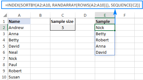
For example, to get 5 unique random names from the list in A2:A10, here's the formula to use:
=INDEX(SORTBY(A2:A10, RANDARRAY(ROWS(A2:A10))), SEQUENCE(5))
For the sake of convenience, you can input the sample size in a predefined cell, say C2, and supply the cell reference to the SEQUENCE function:
=INDEX(SORTBY(A2:A10, RANDARRAY(ROWS(A2:A10))), SEQUENCE(C2))

How this formula works:
Here's a high-level explanation of the formula's logic: the RANDARRAY function creates an array of random numbers, SORTBY sorts the original values by those numbers, and INDEX retrieves as many values as specified by SEQUENCE.
A detailed breakdown follows below:
The ROWS function counts how many rows your data set contains and passes the count to the RANDARRAY function, so it can generate the same number of random decimals:
RANDARRAY(ROWS(A2:C10))
This array of random decimals is used as the "sort by" array by the SORTBY function. As the result, your original data gets shuffled randomly.
From the randomly sorted data, you extract a sample of a specific size. For this, you supply the shuffled array to the INDEX function and request to retrieve the first N values with the help of the SEQUENCE function, which produces a sequence of numbers from 1 to N. Because the original data is already sorted in random order, we do not really care which positions to retrieve, only the quantity matters.
Select random rows in Excel without duplicates
Only works in Excel 365 and Excel 2021 that support dynamic arrays.
To select random rows with no repeats, build a formula in this way:
Where n is the sample size and {1,2,…} are column numbers to extract.
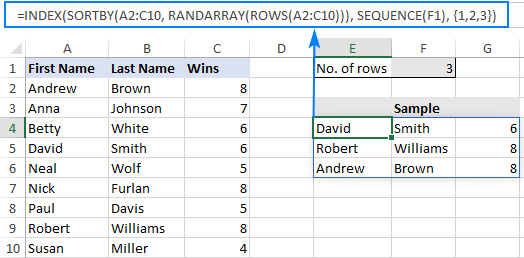
As an example, let's select random rows from A2:C10 without duplicate entries, based on the sample size in F1. As our data is in 3 columns, we supply this array constant to the formula: {1,2,3}
=INDEX(SORTBY(A2:C10, RANDARRAY(ROWS(A2:C10))), SEQUENCE(F1), {1,2,3})
And get the following result:

How this formula works:
The formula works with exactly the same logic as the previous one. A small change that makes a big difference is that you specify both the row_num and column_num arguments for the INDEX function: row_num is supplied by SEQUENCE and column_num by the array constant.
How to do random sampling in Excel 2010 - 2019
As only Excel for Microsoft 365 and Excel 2021 support dynamic arrays, the dynamic array functions used in the previous examples only work in Excel 365. For other versions, you'll have to work out a different solution.
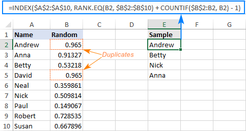
Supposing you want a random selection from the list in A2:A10. This can be done with 2 separate formulas:
- Generate random numbers with the Rand formula. In our case, we enter it in B2, and then copy down to B10:
=RAND() - Extract the first random value with the below formula, which you enter in E2:
=INDEX($A$2:$A$10, RANK.EQ(B2, $B$2:$B$10) + COUNTIF($B$2:B2, B2) - 1) - Copy the above formula to as many cells as many random values you want to pick. In this example, we want 4 names, so we copy the formula from E2 through E5.
Done! Our random sample without duplicates looks as follows:

How this formula works:
Like in the first example, you use the INDEX function to retrieve values from column A based on random row numbers. The difference is in how you get those numbers:
The RAND function fills the range B2:B10 with random decimals.
The RANK.EQ function calculates the rank of a random number in a given row. For example, in E2, RANK.EQ(B2, $B$2:$B$10) ranks the number in B2 against all the numbers in B2:B10. When copied to E3, the relative reference B2 changes to B3 and returns the rank of the number in B3, and so on.
The COUNTIF function finds how many occurrences of a given number there are in the above cells. For instance, in E2, COUNTIF($B$2:B2, B2) checks just one cell - B2 itself, and returns 1. In E5, the formula changes to COUNTIF($B$2:B5, B5) and returns 2, because B5 contains the same value as B2 (please note, this is only to better explain the formula's logic; on a small dataset, chances to get duplicate random numbers are close to zero).
As the result, for all 1st occurrences, COUNTIF returns 1, from which you subtract 1 to keep the original ranking. For 2nd occurrences, COUNTIF returns 2. By subtracting 1 you increment the ranking by 1, thus preventing duplicate ranks.
For example, for B2, RANK.EQ returns 1. As this is the first occurrence, COUNTIF also returns 1. RANK.EQ + COUNTIF gives 2. And - 1 restores the rank 1.
Now, see what happens in case of the 2nd occurrence. For B5, RANK.EQ also returns 1 while COUNTIF returns 2. Adding these up gives 3, from which you subtract 1. As the final result, you get 2, which represents the rank of the number in B5.
The rank goes to the row_num argument of the INDEX function, and it picks the value from the corresponding row (the column_num argument is omitted, so it defaults to 1). This is the reason why it is so important to avoid duplicate ranking. If it were not for the COUNTIF function, RANK.EQ would yield 1 for both B2 and B5, causing INDEX to return the value from the first row (Andrew) twice.
How to prevent Excel random sample from changing
As all randomizing functions in Excel such as RAND, RANDBETWEEN and RANDARRAY are volatile, they recalculate with every change on the worksheet. As the result, your random sample will be continuously changing. To prevent this from happening, use the Paste Special > Values feature to replace formulas with static values. For this, carry out these steps:
- Select all the cells with your formula (any formula containing RAND, RANDBETWEEN or RANDARRAY function) and press Ctrl + C to copy them.
- Right click the selected range and click Paste Special > Values. Alternatively, press Shift + F10 and then V, which is the shortcut for the above-mentioned feature.
For the detailed steps, please see How to convert formulas to values in Excel.
Excel random selection: rows, columns or cells
Works in all versions of Excel 365 through Excel 2010.
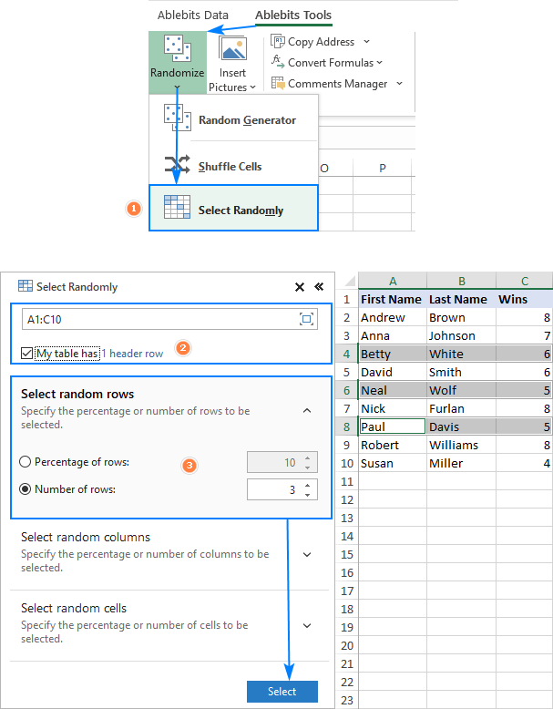
If you have our Ultimate Suite installed in your Excel, then you can do random sampling with a mouse click instead of a formula. Here's how:
- On the Ablebits Tools tab, click Randomize > Select Randomly.
- Select the range from which you want to pick a sample.
- On the add-in's pane, do the following:
- Choose whether you want to select random rows, columns, or cells.
- Define the sample size: that can be a percentage or number.
- Click the Select button.
That's it! As shown in the image below, a random sample is selected directly in your data set. If you'd like to copy it somewhere, just press a regular copy shortcut (Ctrl + C).

That's how to select a random sample in Excel without duplicates. I thank you for reading and hope to see you on our blog next week!
Available downloads
Random sample without duplicates - formula examples (.xlsx file)
Ultimate Suite 14-day fully-functional version (.exe file)
 by
by
3 comments
I'm using this successfully but would like to also add a version of the formula that randomly samples (still without duplicates) but ONLY IF MULTIPLE CRITERIA are met in the corresponding cell in the same row.
This is the formula I'm using
=INDEX(SORTBY(MOICs!$P$21:$P$1193, RANDARRAY(ROWS(MOICs!$P$21:$P$1193))), SEQUENCE($C$11))
For instance, if there's a value in the row P in the sample range that DOES NOT have the correct criteria in the corresponding value in column X, then it should NOT be in the pool to sample from.
Any suggestions?
Hi!
Use the FILTER function to get a list of values that match a certain criterion. From this list, create random samples.
For example,
=INDEX(SORTBY(FILTER(A2:A10,B2:B10=1), RANDARRAY(ROWS(FILTER(A2:A10,B2:B10=1)))), SEQUENCE(D1))
For more information, please visit: Excel FILTER function - dynamic filtering with formulas.
Thank you for posting this formula.