The article looks at how to quickly remove part of text from Excel cells using formulas and inbuilt features.
In this tutorial, we will look at the most common cases of removing characters in Excel. Want to delete specific text from multiple cells? Or maybe strip the first or last character in a string? Or perhaps remove only a specific occurrence of a given character? Whatever your task is, you will find more than one solution for it!
How to remove specific character in Excel
If your goal is to eradicate a certain character from Excel cells, there are two easy ways to do it - the Find & Replace tool and a formula.
Remove character from multiple cells using Find and Replace
Bearing in mind that removing a character is nothing else than replacing it with nothing, you can leverage Excel's Find and Replace feature to accomplish the task.
- Select a range of cells where you want to remove a specific character.
- Press Ctrl + H to open the Find and Replace dialog.
- In the Find what box, type the character.
- Leave the Replace with box empty.
- Click Replace all.
As an example, here's how you can delete the # symbol from cells A2 through A6.
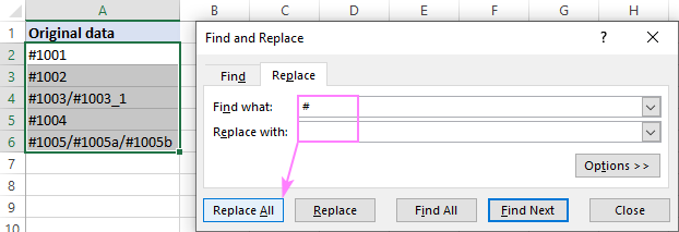
As the result, the hash symbol is removed from all of the selected cells at once, and a pop-up dialog informs you how many replacements have been made:

Tips and notes:
- This method deletes characters directly in your source data. If the result is different from what you expected, press Ctrl + Z to undo the change and get your original data back.
- If you are dealing with alphabetical characters where the letter case matters, click Options to expand the Find and Replace dialog, and then tick the Match case box to perform case-sensitive search.
Remove certain character from string using a formula
To eliminate a specific character from any position is a string, use this generic SUBSTITUTE formula:
In our case, the formula takes this form:
=SUBSTITUTE(A2, "#", "")
Basically, what the formula does is that it processes the string in A2 and replaces each hash symbol (#) with an empty string ("").
Enter the above formula in B2, copy it down through B6, and you will get this result:
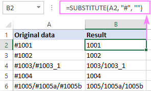
Please pay attention that SUBSTITUTE always returns a text string, even if the result contains only numbers like in cells B2 and B3 (notice the default left alignment typical for text values).
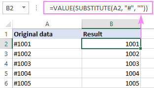
If you want the result to be a number, then wrap the above formula in the VALUE function like this:
=VALUE(SUBSTITUTE(A2, "#", ""))
Or you can perform some math operation that does not change the original value, say add 0 or multiply by 1:
=SUBSTITUTE(A2, "#", "")*1
Delete multiple characters at once
To remove multiple characters with one formula, simply nest SUBSTITUTE functions one into another.
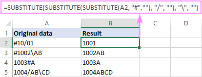
For example, to get rid of a hash symbol (#), forward slash (/) and backslash (\), here's the formula to use:
=SUBSTITUTE(SUBSTITUTE(SUBSTITUTE(A2, "#",""), "/", ""), "\", "")
Tips and notes:
- The SUBSTITUTE function is case-sensitive, please keep that in mind when working with letters.
- If you'd like to have the results as values independent on the original strings, use the Paste special - Values option to replace formulas with their values.
- In situation when there are many different characters to remove, a custom LAMBDA-defined RemoveChars function is a lot more convenient to use.
How to remove certain text from Excel cell
The two methods we used for removing a single character can handle a sequence of characters equally well.
Delete text from multiple cells
To remove specific text from each cell in a selected range, press Ctrl + H to display the Find and Replace dialog, and then:
- Enter the unwanted text in the Find what box.
- Leave the Replace with box blank.

Clicking the Replace All button will do all the replacements in one go:

Remove certain text from cell using a formula
To remove part of a text string, you again use the SUBSTITUTE function in its basic form:
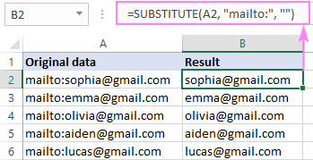
For example, to delete the substring "mailto:" from cell A2, the formula is:
=SUBSTITUTE(A2, "mailto:", "")
This formula goes to B2, and then you drag it down across as many rows as needed:
How to remove Nth instance of a specific character
In situation when you want to delete a certain occurrence of a particular character, define the last optional argument of the SUBSTITUTE function. In the generic formula below, instance_num determines which instance of the specified character should be replaced with an empty string:
For example:
To eradicate the 1st slash in A2, your formula is:
=SUBSTITUTE(A2, "/", "", 1)
To strip the 2nd slash character, the formula is:
=SUBSTITUTE(A2, "/", "", 2)

How to remove first character
To remove the first character from the left side of a string, you can use one of the following formulas. Both do the same thing, but in different ways.
Translated into a human language, the formula says: in the specified cell, take 1 character (num_chars) from the 1st position (start_num), and replace it with an empty string ("").
Here, we subtract 1 character from the total length of the string, which is calculated by the LEN function. The difference is passed to RIGHT for it to extract that number of characters from the end.
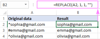
For instance, to remove the first character from A2, the formulas go as follows:
=REPLACE(A2, 1, 1, "")
=RIGHT(A2, LEN(A2) - 1)
The screenshot below shows the REPLACE formula. The RIGHT LEN formula will deliver exactly the same results.
To delete any n characters from the beginning of a string, please see How to remove characters from left in Excel.
How to remove last character
To strip off the last character from the end of a string, the formula is:
The logic is similar to the RIGHT LEN formula from the previous example:
You subtract 1 from the total cell length and serve the difference to the LEFT function, so it can pull that many characters from the beginning of the string.
For instance, you can remove the last character from A2 using this formula:
=LEFT(A2, LEN(A2) - 1)

To delete any n characters from the end of a string, please see How to remove characters from right in Excel.
Remove text after a specific character
To delete everything after a given character, the generic formula is:
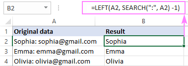
The logic is quite simple: the SEARCH function calculates the position of the specified character and passes it over to the LEFT function, which brings the corresponding number of characters from the beginning. Not to output the delimiter itself, we subtract 1 from the SEARCH result.
For example, to remove text after a colon (:), the formula in B2 is:
=LEFT(A2, SEARCH(":", A2) -1)
For more formula examples, please see Delete text before or after a certain character.
How to remove spaces before and after text in Excel
In text processors such as Microsoft Word, a whitespace before text is sometimes added intentionally to create a balanced and elegant flow for the reader's eye. In spreadsheets programs, leading and trailing spaces may creep unnoticed and cause a lot of problems. Luckily, Microsoft Excel has a special function, named TRIM, to delete extra spaces.
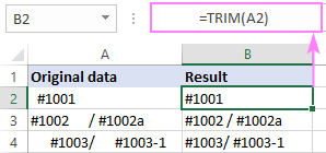
The formula to remove excess spaces from cells is as simple as this:
=TRIM(A2)
Where A2 is your original text string.
As you can see in the image below, it deletes all spaces before text, after text and between words/substrings except for a single space character.
If this simple formula does not work for you, then most likely there are some non-breaking spaces or non-printing characters in your worksheet.
To get rid of them, convert non-breaking spaces into regular spaces with the help of SUBSTITUTE:
SUBSTITUTE(A2, CHAR(160), " ")
Where 160 is the code number of a non-breaking space character ( ).
Additionally, use the CLEAN function to eliminate non-printable characters:
CLEAN(SUBSTITUTE(A2, CHAR(160), " "))
Nest the above construction in the TRIM function, and you'll get a perfect formula to remove spaces before/after text as well as non-breaking spaces and non-printing characters:
=TRIM(CLEAN(SUBSTITUTE(A2, CHAR(160), " ")))
For more information, please see How to remove spaces in Excel.
Remove characters in Excel with Flash Fill
In simple scenarios, Excel's Flash Fill can do you a favor and remove characters or part of text automatically based on the pattern that you provide.
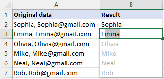
Let's say you have a name and email address in one cell separated by a comma. You want to remove everything after the comma (including the comma itself). To have it done, carry out these steps:
- Insert a blank column to the right of your source data.
- In the first cell of a newly added column, type the value you want to keep (name in our case).
- Start typing the value in the next cell. As soon as Excel determines the pattern, it will show a preview of data to be filled in the below cells following the same pattern.
- Press the Enter key to accept the preview.
Done!
Note. If Excel is unable to recognize a pattern in your data, fill in a couple more cells manually to provide more examples. Also, make sure Flash Fill is enabled in your Excel. If it still does not work, then you'll have to resort to some other method.
Special tools to remove characters or text in Excel
This final section presents our own solutions for removing text from Excel cells. If you love finding simple ways to handle complex challenges, you'll enjoy the handy tools included with Ultimate Suite.
On the Ablebits Data tab, in the Text group, there are three options for removing characters from Excel cells:
- Specific characters and substrings
- Characters in a certain position
- Duplicate characters
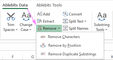
To delete a specific character or substring from selected cells, proceed in this way:
- Click Remove > Remove Characters.
- Select the option best suited to your needs.
- Check or uncheck the Case-sensitive box.
- Hit Remove.
Below are a few examples that cover the most typical scenarios.
Remove specific character
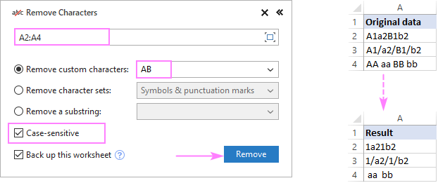
To remove a particular character(s) from multiple cells at once, select Remove custom characters.
As an example, we are deleting all occurrences of the uppercase letters A and B from the range A2:A4:
Delete a predefined character set
To remove a certain set of characters, select Remove character sets, and then choose one of the following options:
- Non-printing characters - strips off any of the first 32 characters in the 7-bit ASCII set (code values 0 through 31) including a tab character, line break, and so on.
- Text characters - removes text and keeps numbers.
- Numeric characters - deletes numbers from alphanumeric strings.
- Symbols & punctuation marks - removes special symbols and punctuation marks such as a period, question mark, exclamation point, comma, etc.

Remove part of text
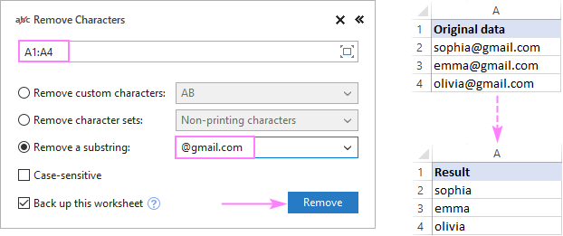
To delete part of a string, choose the Remove a substring option.
For example, to extract usernames from Gmail addresses, we are removing the "@gmail.com" substring:
That's how to remove text and characters from Excel cells. I thank you for reading and look forward to seeing you on our blog next week!
Available downloads
Remove characters in Excel - examples (.xlsm file)
Ultimate Suite - evaluation version (.exe file)
 by
by
26 comments
###########
how to remove or delete using formula or any settings for the above mentioned characteristics or waste values in a table or data sheet.
Hi! If I understand your task correctly, this guide may be helpful: Remove all unwanted characters at once.
Hello there, I have a cell with the below string. I need to remove the numbers but keep the description of words that follow (Architectural Woodwork). Suggestions? Thanks
"06-4000.S
Architectural Woodwork"
Hello Boris!
If I understand correctly, you don't want to delete numbers, but extract all characters after the line break.
Find the line break position using SEARCH function and extract all the following characters using MID function. For example:
=MID(A1,SEARCH(CHAR(10),A1)+1,30)
You can also find useful information in this article: How to remove carriage returns (line breaks) from cells in Excel.
Please am trying to separate a text from a number like Paid -30/09/2024 14:24
I want the paid, date and the time to be separate
Hi! Remove the “-” character from the text using SUBSTITUTE function:
=SUBSTITUTE(A1,"-","")
Then split this text into cells using any of the methods described in these manuals: How to split text string in Excel by comma, space, character or mask or How to split cells in Excel: Text to Columns, Flash Fill and formulas.
You can also use TEXTSPLIT function:
=TEXTSPLIT(SUBSTITUTE(A1,"-","")," ")
Read more: TEXTSPLIT function in Excel: split text strings by delimiter.
Hello,
I am trying to separate or remove just the date on one cell tried textafter,textsplit still doesn't work
example in one cell value includes date and time ==> "4/1/2024 05:00 AM" - I just want to remove the date or move it to another cell and remain just the time.
Please help
Thank you
Hello Navin!
Unfortunately, I don't know what result you want: "05:00 AM", "05:00" or 05:00 as time.
To extract the text between the second and third spaces "05:00", you can use these guidelines: Split string by comma, semicolon, slash, dash or other delimiter.
The formula might look like this:
=MID(A2, SEARCH(" ",A2) + 1, SEARCH(" ",A2,SEARCH(" ",A2)+2) - SEARCH(" ",A2) - 1)
With this formula, you extract the time as text.
With the TEXTBEFORE and TEXTAFTER functions, you can get the time as text:
=TEXTAFTER(A2," ",1)
or
=TEXTBEFORE(TEXTAFTER(A2," ",1)," ")
To get the time from the text, you can use the TIMEVALUE function:
=TIMEVALUE(TEXTBEFORE(TEXTAFTER(A2," ",1)," "))
=TIMEVALUE(MID(A2,SEARCH(" ",A2)+1,SEARCH(" ",A2,SEARCH(" ",A2)+2)-SEARCH(" ",A2)-1))
If the format of this text matches your system date and time settings, you can convert the text to date and time using a mathematical operation and then get the time value:
=(MOD(--A2,1))
Set the desired time format in the formula cell.
000001 - I need to replace the first zero in the string to a 1
Hi! Find the position of the first "0" using the SEARCH function and replace it with a "1" using the REPLACE function. Try this formula:
=REPLACE(A1,SEARCH("0",A1),1,1)
hi sir alexander,
i have 123400000567890 in A1, i want to replace zeros with "-" like this: 1234-567890
sometimes zeros changes like this, 432100000009876 and i want to replace it with 4321-9876
or sometimes like this, 789000000012345 and replace it with 7890-12345
number in A1 is always 15 digits and i want to replace consecutive zeros after the 4 digits with "-"
is it possible?? thanks in advance
To replace characters in a string by a pattern, you can use regular expressions and the custom RegExpReplace function.
For example,
=LEFT(A1,4)&RegExpReplace(MID(A1,5,20), "0{3,10}", "-")
We extract the first 4 characters from the text. In the rest of the text, starting from the fifth character, the RegExpReplace function looks for a group of zeros from 3 to 10 and replaces them with "-".
For more information, please visit: Excel Regex to find and replace strings using regular expressions. I hope my advice will help you solve your task.
If have a line like this " @Raja @rani @john @will you are so sweeet!. so I want to delete the name after @ with @ sign. Be clear I want to delete the name with @. Means output will be only " you are so sweeet!". How I delete all the name at a time so only meaningful sentence will output.?
Hi!
To find all substrings in the text that match the pattern and remove them, the custom function RegExpReplace is used. It is used to replace the text. To remove substrings matching the pattern, use an empty string ("") to replace them.
You can find the examples and detailed instructions here: Excel Regex to remove certain characters or text from strings.
@.*?\s\b - pattern
=RegExpReplace(A1, "@.*?\s\b", "", 1) - formula
I recommend paying attention to the Regex tools. You can find, extract, remove, or replace strings that match a regex pattern you enter. It is available as a part of our Ultimate Suite for Excel that you can install in a trial mode and check how it works for free.
Hello Alex and albeit team, do you mind helping me write a formula based on these sets of data?
so the original data would be: Social Media Group(socialmediagroup.com)
and the result I'm expecting: socialmediagroup.com
I used this formula
=RIGHT(C3;SEARCH("(";C3)-1)
even tried the ones with "LEN", I cannot seem to find the solution.
thank you
Hello!
To extract text between two characters, you can use this article's recommendations: Extract text between two characters in Excel.
=MID(A1,SEARCH("(",A1)+1,SEARCH(")",A1)-SEARCH("(",A1)-1)
or
=TEXTBEFORE(TEXTAFTER(A1, "("), ")")
This should solve your task.
Is there a way to remove three words from an excel spreadsheet. the three words needing to be removed from each cell are all of different lengths but are all separated by a space
Hello!
Try to use these recommendations: Regex to remove certain characters or text in Excel.
Hello :)
I need to remove the last digits in a string of text eg “Thomas Andrew jeffery 5555” the length of number at the end may vary
Hello!
Please check the formula below, it should work for you:
=LEFT(A1,SEARCH("#",SUBSTITUTE(A1," ","#",LEN(A1)-LEN(SUBSTITUTE(A1," ",""))))-1)
For more information, please read: How to split text in Excel using formulas.
To extract all the text before a specific character, you can use the Excel TEXTBEFORE function.
=TEXTBEFORE(A1," ",LEN(A1)-LEN(SUBSTITUTE(A1," ","")))
I hope my advice will help you solve your task.
Hi,
I have the following text on a cell: Matthew Stafford\StafMa00
and I need to only have Last Name, First Name (Stafford, Matthew)
Thanks so much!
Hello!
Excel substring functions to extract text from cell
=LEFT(A1,SEARCH("\",A1)-1)
You can also use the new function TEXTBEFORE:
=TEXTBEFORE(A1,"\")
Hi, hope you can help me.
I have a sheet that contains cells with data I do not want. Such as:
"Save"
"View profile"
"Add Phil Nock to selection"
etc...
They all have a pattern, in the sense that the cells I do not want all have a pattern throughout the sheet, either containing a whole word in a cell like "add" or with text that follows the common word "add Phil Nock..."
I have a list of common words that are found after i have sorted my list to satisfaction, but have no clue how to "Find" a word in a cell, and "remove" who whole cell if that word is found, whether it is in whole or in part "add" or "add Phil..."
Hi!
Try using the Excel Find and Select tool. Try to use the recommendations described in this guide: Excel Find and Replace with wildcards. To remove, use replace with nothing.
Hope you’ll find this information helpful.
Hi I have a string of reviews mined from a review site like this:
Trish Mar 30 2022 9:09 pm
This series moved me to tears quite a few times. BRILLIANT acting by all actors and actresses involved. Thank You for your hard work. CHEERS!
How do I remove the name and date/time for all 1518 rows?
Hello!
Use the SEARCH function to find the position of the first space and line break. Extract text at these positions and concatenate strings.
Please try the following formula:
=LEFT(A1,SEARCH(" ",A1))&MID(A1,SEARCH(CHAR(10),A1),200)