The tutorial explains how to search for duplicates in Excel. You will learn a few formulas to identify duplicate values or find duplicate rows with or without first occurrences. You will also learn how to count instances of each duplicate record individually and find the total number of dupes in a column, how to filter out duplicates, and more.
While working with a large Excel worksheet or consolidating several small spreadsheets into a bigger one, you may find lots of duplicate rows in it. In one of our previous tutorials, we discussed various ways to compare two tables or columns for duplicates.
And today, I'd like to share a few quick and effective methods to identify duplicates in a single list. These solutions work in all versions of Excel 365, Excel 2021, Excel 2019, Excel 2016, Excel 2013 and lower.
How to identify duplicates in Excel
The easiest way to detect duplicates in Excel is using the COUNTIF function. Depending on whether you want to find duplicate values with or without first occurrences, there's going to be a slight variation in the formula as shown in the following examples.
How to find duplicate records including 1st occurrences
Supposing you have a list of items in column A that you want to check for duplicates. These can be invoices, product Id's, names or any other data.
Here's a formula to find duplicates in Excel including first occurrences (where A2 is the topmost cell):
=COUNTIF(A:A, A2)>1
Input the above formula in B2, then select B2 and drag the fill handle to copy the formula down to other cells:
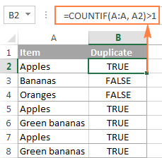
As you can see in the screenshot above, the formula returns TRUE for duplicate values and FALSE for unique values.
Note. If you need to find duplicates in a range of cells rather than in an entire column, remember to lock that range with the $ sign. For example, to search for duplicates in cells A2:A8, use this formula:
=COUNTIF($A$2:$A$8, A2)>1
For a duplicate formula to return something more meaningful than the Boolean values of TRUE and FALSE, enclose it in the IF function and type any labels you want for duplicate and unique values:
=IF(COUNTIF($A$2:$A$8, $A2)>1, "Duplicate", "Unique")
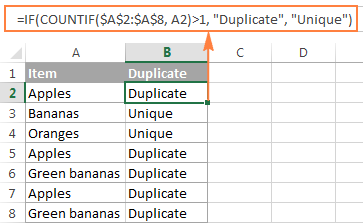
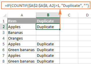
In case, you want an Excel formula to find duplicates only, replace "Unique" with an empty string ("") like this:
=IF(COUNTIF($A$2:$A$8, $A2)>1, "Duplicate", "")
The formula will return "Duplicates" for duplicate records, and a blank cell for unique records:
How to search for duplicates in Excel without 1st occurrences
In case you plan to filter or remove duplicates after finding them, using the above formula is not safe because it marks all identical records as duplicates. And if you want to keep the unique values in your list, then you cannot delete all duplicate records, you need to only delete the 2nd and all subsequent instances.
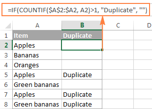
So, let's modify our Excel duplicate formula by using absolute and relative cell references where appropriate:
=IF(COUNTIF($A$2:$A2, $A2)>1, "Duplicate", "")
As you can see in the following screenshot, this formula does not identity the first occurrence of "Apples" as duplicate:
How to find case-sensitive duplicates in Excel
In situations when you need to identify exact duplicates including the text case, use this generic array formula (entered by pressing Ctrl + Shift + Enter):
At the heart of the formula, you use the EXACT function to compare the target cell with each cell in the specified range exactly. The result of this operation is an array of TRUE (match) and FALSE (not match), which is coerced to an array of 1's and 0's by the unary operator (--). After that, the SUM function adds up the numbers, and if the sum is greater than 1, the IF function reports a "Duplicate".
For our sample dataset, the formula goes as follows:
=IF(SUM((--EXACT($A$2:$A$8,A2)))<=1,"","Duplicate")
As shown in the screenshot below, it treats lowercase and uppercase as different characters (APPLES is not identified as a duplicate):

Tip. If you are using Google spreadsheets, the following article might be helpful: How to find and remove duplicates in Google Sheets.
How to find duplicate rows in Excel
If your aim is to dedupe a table consisting of several columns, then you need a formula that can check each column and identify only absolute duplicate rows, i.e. rows that have completely equal values in all columns.
Let's consider the following example. Supposing, you have order numbers in column A, dates in column B, and ordered items in column C, and you want to find duplicate rows with the same order number, date and item. For this, we are going to create a duplicate formula based on the COUNTIFS function that allows checking multiple criteria at a time:
To search for duplicate rows with 1st occurrences, use this formula:
=IF(COUNTIFS($A$2:$A$8,$A2,$B$2:$B$8,$B2,$C$2:$C$8,$C2)>1, "Duplicate row", "")
The following screenshot demonstrates that the formula really locates only the rows that have identical values in all 3 columns. For example, row 8 has the same order number and date as rows 2 and 5, but a different item in column C, and therefore it is not marked as duplicate row:
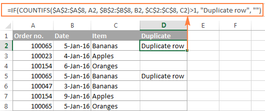
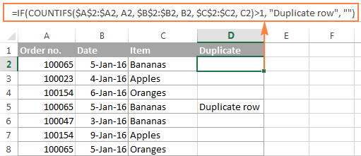
To show duplicate rows without 1st occurrences, make a little adjustment to the above formula:
=IF(COUNTIFS($A$2:$A2,$A2,$B$2:$B2,$B2,$B$2:$B2,$B2,$C$2:$C2,$C2,) >1, "Duplicate row", "")
How to count duplicates in Excel
If you want to know the exact number of identical records in your Excel sheet, use one of the following formulas to count duplicates.
Count instances of each duplicate record individually
When you have a column with duplicated values, you may often need to know how many duplicates are there for each of those values.
To find out how many times this or that entry occurs in your Excel worksheet, use a simple COUNTIF formula, where A2 is the first and A8 is the last item of the list:
=COUNTIF($A$2:$A$8, $A2)
As demonstrated in the following screenshot, the formula counts the occurrences of each item: "Apples" occurs 3 times, "Green bananas" - 2 times, "Bananas" and "Oranges" only once.

If you want to identify 1st, 2nd, 3rd, etc. occurrences of each item, use the following formula:
=COUNTIF($A$2:$A2, $A2)

In a similar manner, you can count the occurrences of duplicated rows. The only difference is that you will need to use the COUNTIFS function instead of COUNTIF. For example:
=COUNTIFS($A$2:$A$8, $A2, $B$2:$B$8, $B2)

Once the duplicate values are counted, you can hide unique values and only view duplicates, or vice versa. To do this, apply Excel's auto-filter as demonstrated in the following example: How to filter out duplicates in Excel.
Count the total number of duplicates in a column(s)
The easiest way to count duplicates in a column is to employ any of the formulas we used to identify duplicates in Excel (with or without first occurrences). And then you can count duplicate values by using the following COUNTIF formula:
=COUNTIF(range, "duplicate")
Where "duplicate" is the label you used in the formula that locates duplicates.
In this example, our duplicate formula takes the following shape:
=COUNTIF(B2:B8, "duplicate")
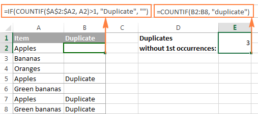
Another way to count duplicate values in Excel by using a more complex array formula. An advantage of this approach is that it does not require a helper column:
=ROWS($A$2:$A$8)-SUM(IF( COUNTIF($A$2:$A$8,$A$2:$A$8)=1,1,0))
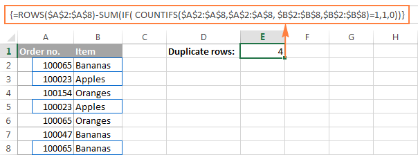
Because it's an array formula, remember to press Ctrl + Shift + Enter to complete it. Also, please keep in mind that this formula counts all duplicate records, including first occurrences:

To find the total number of duplicate rows, embed the COUNTIFS function instead of COUNTIF in the above formula, and specify all of the columns you want to check for duplicates. For example, to count duplicate rows based on columns A and B, enter the following formula in your Excel sheet:
=ROWS($A$2:$A$8)-SUM(IF( COUNTIFS($A$2:$A$8,$A$2:$A$8, $B$2:$B$8,$B$2:$B$8)=1,1,0))
How to filter duplicates in Excel
For easier data analysis, you may want to filter your data to only display duplicates. In other situations, you may need the opposite - hide duplicates and view unique records. Below you will find solutions for both scenarios.
How to show and hide duplicates in Excel
If you want to see all duplicates at a glance, use one of the formulas to find duplicates in Excel that better suits your needs. Then select your table, switch to the Data tab, and click the Filter button. Alternatively, you can click Sort & Filter > Filter on the Home tab in the Editing group.
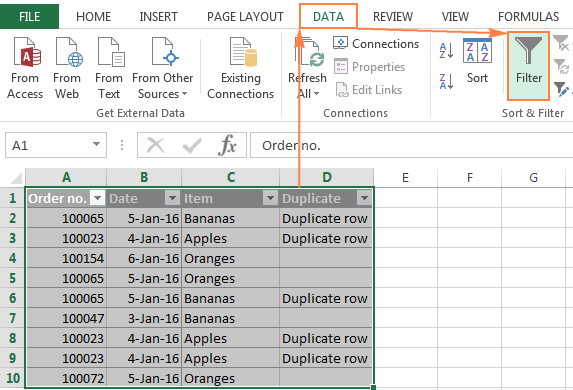
Tip. To have filtering enabled automatically, convert your data to a fully-functional Excel table. Just select all data and press the Ctrl + T shortcut.
After that, click the arrow ![]() in the header of the Duplicate column and check the "Duplicate row" box to show duplicates. If you want to filter out, i.e. hide duplicates, select "Unique" to view only unique records:
in the header of the Duplicate column and check the "Duplicate row" box to show duplicates. If you want to filter out, i.e. hide duplicates, select "Unique" to view only unique records:

And now, you can sort duplicates by the key column to group them for easier analysis. In this example, we can sort duplicate rows by the Order number column:
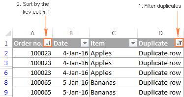
How to filter duplicates by their occurrences
If you want to show 2nd, 3rd, or Nth occurrences of duplicate values, use the formula to count duplicate instances we discussed earlier:
=COUNTIF($A$2:$A2, $A2)
Then apply filtering to your table and select only the occurrence(s) you want to view. For example, you can filter the 2nd occurrences like in the following screenshot:

To display all duplicate records, i.e. occurrences greater than 1, click the filter arrow in the header of the Occurrences column (the column with the formula), and then click Number Filters > Greater Than.
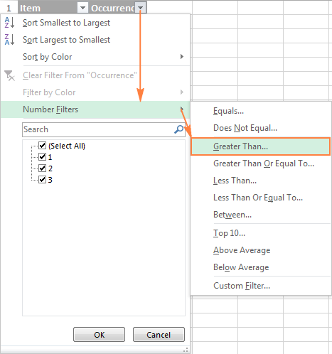
Select "is greater than" in the first box, type 1 in the box next to it, and click the OK button:

In a similar manner, you can show 2nd, 3rd and all subsequent duplicate occurrences. Just type the required number in the box next to "is greater than".
Highlight, select, clear, delete, copy or move duplicates
After you've filtered duplicates like demonstrated above, you have a variety of choices to deal with them.
How to select duplicates in Excel
To select duplicates, including column headers, filter them, click on any filtered cell to select it, and then press Ctrl + A.
To select duplicate records without column headers, select the first (upper-left) cell, and press Ctrl + Shift + End to extend the selection to the last cell.
Tip. In most cases, the above shortcuts work fine and select filtered (visible) rows only. In some rare cases, mostly on very large workbooks, both visible and invisible cells may get selected. To fix this, use one of the above shortcuts first, and then press Alt + ; to select only visible cells, ignoring hidden rows.
How to clear or remove duplicates in Excel
To clear duplicates in Excel, select them, right click, and then click Clear Contents (or click the Clear button > Clear Contents on the Home tab, in the Editing group). This will delete the cell contents only, and you will have empty cells as the result. Selecting the filtered duplicate cells and pressing the Delete key will have the same effect.
To remove entire duplicate rows, filter duplicates, select the rows by dragging the mouse across the row headings, right click the selection, and then choose Delete Row from the context menu.

How to highlight duplicates in Excel
To highlight duplicate values, select the filtered dupes, click the Fill color button ![]() on the Home tab, in the Font group, and then select the color of your choosing.
on the Home tab, in the Font group, and then select the color of your choosing.
Another way to highlight duplicates in Excel is using a built-in conditional formatting rule for duplicates, or creating a custom rule specially tailored for your sheet. Experienced Excel users won't have any problem with creating such a rule based on the formulas we used to check duplicates in Excel. If you are not very comfortable with Excel formulas or rules yet, you will find the detailed steps in this tutorial: How to highlight duplicates in Excel.
How to copy or move duplicates to another sheet
To copy duplicates, select them, press Ctrl + C, then open another sheet (a new or existing one), select the upper-left cell of the range where you want to copy the duplicates, and press Ctrl + V to paste them.
To move duplicates to another sheet, perform the same steps with the only difference that you press Ctrl + X (cut) instead of Ctrl + C (copy).
Duplicate Remover - fast and efficient way to locate duplicates in Excel
Now that you know how to use duplicate formulas in Excel, let me demonstrate you another quick, efficient and formula-free way - Duplicate Remover for Excel.
This all-in-one tool can search for duplicate or unique values in a single column or compare two columns. It can find, select and highlight duplicate records or entire duplicate rows, remove found dupes, copy or move them to another sheet. I think an example of practical use is worth many words, so let's get to it.
How to find duplicate rows in Excel in 2 quick steps
To test the capabilities of our Duplicate Remover add-in, I've created a table with a few hundred rows that looks like follows:

As you see, the table has a few columns. The first 3 columns contain the most relevant information, so we are going to search for duplicate rows based solely on the data in columns A - C. To find duplicate records in these columns, just do the following:
- Select any cell within your table and click the Dedupe Table button on the Excel ribbon. After installing our Ultimate Suite for Excel, you will find it on the Ablebits Data tab, in the Dedupe group.
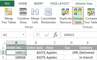
- The smart add-in will pick up the entire table and ask you to specify the following two things:
- Select the columns to check for duplicates (in this example, these are the Order no., Order date and Item columns).
- Choose an action to perform on duplicates. Because our purpose is to identify duplicate rows, I've selected the Add a status column

Apart from adding a status column, an array of other options are available to you:
- Delete duplicates
- Color (highlight) duplicates
- Select duplicates
- Copy duplicates to a new worksheet
- Move duplicates to a new worksheet
Click the OK button and wait for a few seconds. Done!
As you can see in the below screenshot, all of the rows that have identical values in the first 3 columns have been located (first occurrences are not identified as duplicates).

If you want more options to dedupe your worksheets, use the Duplicate Remover wizard that can find duplicates with or without first occurrences as well as unique values. The detailed steps follow below.
Duplicate Remover wizard - more options to search for duplicates in Excel
Depending on a particular sheet you are working with, you may or may not want to treat the first instances of identical records as duplicates. One possible solution is using a different formula for each scenario, as we discussed in How to identify duplicates in Excel. If you are looking for a fast, accurate and formula-free method, try the Duplicate Remover wizard:
- Select any cell within your table and click the Duplicate Remover button on the Ablebits Data tab. The wizard will run and the entire table will get selected.

- On the next step, you are presented with the 4 options to check duplicates in your Excel sheet:
- Duplicates without 1st occurrences
- Duplicates with 1st occurrences
- Unique values
- Unique values and 1st duplicate occurrences
For this example, let's go with the second option, i.e. Duplicates + 1st occurrences:

- Now, select the columns where you want to check duplicates. Like in the previous example, we are selecting the first 3 columns:
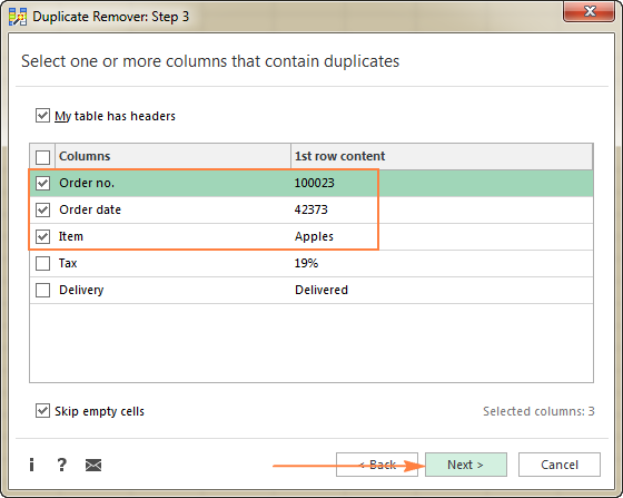
- Finally, choose an action you want to perform on duplicates. As is the case with the Dedupe Table tool, the Duplicate Remover wizard can identify, select, highlight, delete, copy or move duplicates.
Because the purpose of this tutorial is to demonstrate different ways to identify duplicates in Excel, let's check the corresponding option and click Finish:

It only takes a fraction of a second for the Duplicate Remover wizard to check hundreds of rows, and deliver the following result:

No formulas, no stress, no errors - always swift and impeccable results :)
If you are interested to try these tools to find duplicates in your Excel sheets, you are most welcome to download an evaluation version below. Your feedback in comments will be greatly appreciated!
Available downloads
Identify Duplicates - formula examples (.xlsx file)
Ultimate Suite - trial version (.exe file)
 by
by
260 comments
Dear Sir/Madam,
Is there a way to find duplicate values in a single cell in MS-Excel? I'm working on a CSV file where there are duplicate values occurring in a single cell only. Can you please help?
Hello!
You need to split the text from this cell into other cells. You can then look for duplicates in these cells.
I recommend using the Split Cells tool for this.
Duplicate Remover will help you find duplicates in cells.
It is available as a part of our Ultimate Suite for Excel that you can install in a trial mode and check how it works for free.
How to find last 4 digit duplicate value and marked. is there any formula. e.g.
JVC2020TDL2946
BV2020TDL2946
JVC2020TDL2947
BV2020TDL2947
JV2020TDL0224
JV2020TDL0225
Hello!
You can extract the last 4 digits into a separate column using the RIGHT function. Then look for duplicates in that column as described in the tutorial above.
I hope this will help, otherwise please do not hesitate to contact me anytime.
Thanks Sir
for your reply and i have also tried this option it will work properly.
I know that this is old but the easiest solution would be to highlight a column, go to conditional formatting->highlight cell rules, then duplicates. After that, just filter by color.
To rmove them, there is a built in button in excel, under the data tab.
How to choose repeated number example for this case:
12344445678910444. The correct answer is 4
Hi, I need to modify the formula that extracts ONLY duplicates from column to make it able to work from the first row.
=IFERROR(INDEX(A$2:A$16,MATCH(1,COUNTIF($A$1:A1,A$2:A$16)=0)*COUNTIF(A$2:A$16,A$2:A$16)>=2)),0)),"")
As you can see it doesn't allow to be placed in the first row due to cell reference problem in this part COUNTIF($A$1:A1,A$2:A$16).
Is there any alternative option?
Hi
I hope you are doing very well.
Your solutions are very helpful.
Thanks a lot.
hi, how to find duplicate from 2 sheets and highlight with color
Hello!
All the recommendations you need are listed in the article above. Make external references to another sheets of your workbook correctly as described in this guide.
I am trying to count how many duplicate names are found in Col A. I have 600 plus rows and I just want the count each time I find a duplicate value. I tried
Column B
=COUNTIF($A$2:$A$800, $A2)
Column C
=IF(COUNTIF($A$2:$A$800, $A2)>1, "Duplicate", "Unique")
But I only return 722 value in Column, and only Duplicate in Column C (used to remove Duplicate, just leave one count total.)
Im looking for:
Appels 121
Grapes 253
Bananas 10
Oranges 400
Is this possible? Any kind help?
Hi,
I don't really understand what you want to find. To remove duplicates, it is best to use a formula that ignores the first occurrence of the value. See "How to search for duplicates in Excel without 1st occurrences". To remove duplicates, I recommend using Duplicate Remover Toolkit for Excel. It is available as a part of our Ultimate Suite for Excel that you can install in a trial mode and check how it works for free.
If this is not what you want, please describe the problem in more detail. I will try to help.
Hi,
I would need some help regarding this issues:
1. I have a list with names, I had found the duplicates. My task is: Using a single formula, detect all of the duplicates in the above list. If the term has already appeared in the list, then your formula should display it on the same row, if the term has not already appeared on the list then your formula should display N/A.
Name
Cristina
Ioana
Florin
George
Cristina
Cosmin
Neculai
Alina
Florentina
Andreea
Laura
Alina
2. I need a formula for completing this task: Create a formula that returns only the characters that appear after "X" for the given character strings. The same formula must work for the whole column!
Example: 45629X421 421
I found the formula for task 2.
Any thoughts for the 1st task?
Thanks!
Hello!
I hope you have studied the recommendations in the tutorial above. It contains answers to your question.
To return all characters after "X" use the formula
=MID(B1,SEARCH("X",B1,1)+1,100)
I hope it’ll be helpful.
How do i get collegue names if website duplicates. Let say first 3 people are at same company (same website) So i need to get collegue name such as
Sam - Nick
Nick - David
David - Sam
How do i get them.
Full Name Collegue Name Website
Sam abc.com
Nick abc.com
David abc.com
Peter 123.com
Ann 123.com
Hello!
If I understand your task correctly, the following formula should work for you:
{=IFERROR(INDEX($B$2:$B$12, SMALL(IF($D2=$A$2:$A$12, ROW($B$2:$B$12)-1,""), COLUMN()-4)),"")}
This is an array formula and it needs to be entered via Ctrl + Shift + Enter, not just Enter. Line 1 is the title of the table. Column A is a list of websites. Column B is a list of names. Column D is the website where you want to find the names of colleagues.
You can read more about this formula in the article: How to VLOOKUP multiple values in Excel
You can combine names in one cell with delimiters using the formula
=TEXTJOIN("-",TRUE,J2:N2)
I hope my advice will help you solve your task. If something is still unclear, please feel free to ask.
Hello,
sorry, how to find the last duplicate value in row ,
such as:
A B C D
2 4 3 2
i want to find the number "2" that is from column "D"
tnx..
Hello!
If I understand your task correctly, the following formula should work for you:
=IFERROR(INDEX((IF(COUNTIF(A1:F1,A1:F1)>1,A1:F1,"")),,MATCH(TRUE,(IF(COUNTIF(A1:F1,A1:F1)>1,A1:F1,""))<>"",0)),"")
I hope I answered your question. If something is still unclear, please feel free to ask.
extremely killer tricks.... Brilliant.... Many wishes for you and best of luck...
how can I set formula to move any duplicates document id to next 3 columns in excel? thanks
document id: 1st allocation id 2nd allocation id 3rd allocation ID
12345
23456
12356
11236
23456
23562
89712
12345
12346
12356
Hello!
Sorry, it's not quite clear what you are trying to achieve. I don't see any pattern in your numbers. Could you please describe it in more detail? What result do you want to get?
I am creating a quiz bank. I want to find duplicates within a row and then be able to copy the formula down a column. I tried using the formula =IF(COUNTIF(C1:I1,), "duplicate", ""). However it only returns duplicates of the first cell. I need to know if ANY of the cells in that row are duplicates. Please help!
Sorry I just realized the formula i put in above is not the formula I am using. It is =if(countif(C1:I1,C1)>1 "duplicate", "")
Hello!
If I got you right, the formula below will help you with your task:
=IF(SUM(--(COUNTIF(C1:I1,C1:I1)>1)) > 0,"duplicate","")
After that, you can copy this formula down along the column.
I hope it’ll be helpful.
It works perfectly! Thank you SOOOOOOOO much!
If the range is not continious, example A1:A5 and B1:B15 then how to check if the 15 values in these cells have duplicate or not
Hello!
Unfortunately, Excel cannot search data in multiple data ranges at the same time.
Hey
How to paste data in a merge cell
Help me if u know
Hello!
I’m sorry but your task is not entirely clear to me.
Please describe your problem in more detail. Write an example of the source data and the result you want to get. It’ll help me understand it better and find a solution for you. Thank you.
Quick Question, Is there a way to set the 1st row of duplicate records to "Parent"
I am using this formula: =IF(COUNTIFS($A$2:$A,A2,$B$2:$B,B2,$C$2:$C,C2)>1,"Child","Parent")
Row 1 - Parent
Row 2 - Child
Row 3 - Child
instead of
Row 1 - Child
Row 2 - Child
Row 3 - Child
Help is greatly appreciated.
Hello!
If I understand your task correctly, you need to set the first occurrence of a duplicate as Parent" marking the rest of them as "Child".
Assuming that your table has no header, here is the right formula for you:
=IF(COUNTIF(A1:$A$26,A1)>1, IF(AND(COUNTIF(A1:$A$26,A1)>1, MATCH(A1,$A$1:$A$26,0)=ROW(A1)), "Parent","Child"),"")
If however, there is a 1-line header, the formula should be modified a little to look like the one below:
=IF(COUNTIF(A2:$A$27,A2)>1, IF(AND(COUNTIF(A2:$A$27,A2)>1, MATCH(A2,$A$2:$A$27,0)=ROW(A2)-1), "Parent","Child"),"")
Hope this is exactly what you need.
ok I have an excel worksheet that I want to add a formula to catch duplicates throughout the worksheet. I don't want the 1st selected column ex:A2 to change I want it to carry down to where it catches any above it, Say I am on row A 15 I want it to look at rows A2-A14 to make sure the information I added in A15 wasn't on any above it. Can you help with this please?
Good Afternoon!
I have a workbook spreadsheet (SP1) that is pulling data from another workbook spreadsheet (SP2) using an if statement formula. In SP2, column A, I'm pulling data from SP1, column G. I would like to highlight the row in SP2 if a duplicate is found in column A. However, I'm not sure if I can do that with there already being a formula in each cell.
To better clarify my question - Is there a way to highlight a row when the data pulled in column A duplicates, and to not highlight if no data is pulled or the result is "false".
My issue right now is that because there is a formula in every cell when I use conditional formatting it ends up highlighting the entire workbook. I only want it to highlight if column A shows a duplicate result (A1 formula result shows: a, A5 formula result shows: a).
Thanks, Svetlana
It was awesome.
Is there a way to find the exact location (using Index and Match) next to the first, second (and so on) duplicate value? Suppose Mary 100 and Donald 100 in a long list of names in column A and values in column B. Would it be possible using Index/Match to put "Mary" and "Donald" in the same order in Column C?
Hi,
I need to flag 1st duplicate and 2nd duplicate till nth duplicate with respect to date.
for ex: 01/01/2010 is having data with duplicates and using COUNTIF it can return 1st duplicate and then 02/01/2020 is having same data and I need to flag second duplicate vice versa.
I am using below formula
"{=IF(COUNTIF($A$3:A3,A3)>1,"NX","X")}
here "X" return with 1st duplicate value
I need to find out the duplicates for the below...anybosy pl help me..
For example..
Apple
Banana
Apple
Banana
Apple
Banana
Apple
Apple
In the last 2 rows, word apple repeated...this need to be find out in the consecutive list....1 :1 ratio only allowed...pl help
for same exact work or number finding duplicate is ok
but i am looking for something like this
apple,banana
apple,mango
mango,banana
how to find same word in a cell for whole column
Hi,
How can i get duplicate value or text & unique value or text by using reference in excel.
Thank you very much, I have gained a lot and I can identify easily the duplicates for following the formulas.
Abdinasir
Wondering if there is a formula to begin counting up every there is a change in the name column; as so:
Name #
1 1
1 2
1 3
2 1
2 2
2 3
3 1
3 2
3 3
4 1
5 1
6 1
6 2
7 1
7 2
7 3
8 1
8 2
8 3
9 1
9 2
10 1
11 1
11 2
11 3
Please how do I check for duplicate interval. eg
hole_id depth_from depth_to
NGC12-018 0 1.5
NGC12-018 1.5 2.3
NGC12-018 2.3 3
NGC12-018 3 8.2
NGC12-018 8.2 10.7
NGC12-018 10.7 17.3
NGC12-018 17.3 20.6
NGC12-018 20.6 23.5
NGC12-018 20.6 23.5
NGC12-018 23.5 27.9
NGC12-018 27.9 31.7
NGC12-018 31.7 36.7
NGC12-018 36.7 43.4
NGC12-018 36.7 43.4
NGC12-018 43.4 48.2
NGC12-018 48.2 49.5
NGC12-018 49.5 64.5
NGC12-018 64.5 67.5
NGC12-018 67.5 72.6
NGC12-018 72.6 81
NGC12-018 81 86.55
NGC12-018 86.55 90
I am working on a list of not duplicate text cells but some are close.
I want to know how to only find the cells that are incorrect.
How do I do that?
Here is an example.
9086264 SENSOR RTD JACKET HEATING TETRA PAK ALLM O-RING 9531-4040-591 FALSE
9086266 SEAL CYLINDER CLOSING TOOL SCRAPER ROD 9531-6131-516 FALSE
9086267 ARM CASE SIDE CLOSING GASKET 9531-6130-516 FALSE
9086270 TRAP STEAM DISC TD42H SPIRAX SARCO O-RING 9531-4021-591 FALSE
I have a list of 20,000 items that I can not go through indivually. I just want to make sure the first few characters match.
Kindly Solve My Query in below there is two value in a saprate cells , i wants comman value in output cell.
Value 1 Value 2 Output (Comman No.)
21452 23652 25
Hi, I'm using the duplicate formula but trying to add an index part so that it shows up the duplicate reference. Where am I going wrong and how do I correct it? I have: =INDEX(E:E(IF(COUNTIF(F:F,[@WON])>1,"Duplicate","")),0)
I want to show the contents of the duplicate cell from column E, if it has the same contents as another cell in column F. So if row 3 has the same column F value as row 5, I want B3 to show the cell value from E5.
I hope this makes sense.
Thanks
016230240
016259070
012350891
If i would like to add a 6 in front of above number only, example 016 become 6016230240 , the back of 0 will appear 6 also if i find 0 and replace by 6, however i just like to have 6 infront of the number, what is the the process , pls help, thank you..
Hi,
How can I distinguish repeating brand names? For example:
Gillette --> Gillette 1
Gillette --> Gillette 2
Pantene --> Pantene 1
Gillette --> Gillette 3
Head & Shoulders --> Head & Shoulders 1
Pantene --> Pantene 2
How can i arrange the Values of duplicate attendance number from below
Attendace Value
168755 41759002
168755 41704067
197119 40316326
197119 40811539
204786 41446987
204786 41025753
285943 41696614
285943 41232806
181907 40538480
181907 40117598
986727 40450723
986727 41072614
768565 40098263
768565 40403845
693968 40455014
693968 40987284
998263 40044440
998263 40928398
366864 41736203
366864 41644887
837218 40222382
837218 40621245
837218 4063258
to
Attendance Value 1 Value 2 Value3
168755 41759002 41704067
197119 40316326 40811539
204786 41446987 41025753
285943 41696614 41232806
181907 40538480 40117598
986727 40450723 41072614
768565 40098263 40403845
693968 40455014 40987284
998263 40044440 40928398
366864 41736203 41644887
837218 40222382 40621245 4063258
Hi
am saikat patra from Howrah in west bengal.
Can anyone help me about if count formula details given below.
colum 1 colum 2
78120 above10days
78121 above10days
78122 abovel0days
78560 above5days
78121 above10days
How to count colum 2 tex wise to colum 1 shipment no without duplicate.
ans should be if above10days basis is "3".
please help me and very much gladfull to you for this.
Hi,
how can i get the duplication data for example i want the excel to read the data from 6 last alphabet of an email.
Highlight duplicate values across multiple worksheets.
I have a workbook with four worksheets. We are clearing out a storage center and listing the bins on worksheet "Empty Bins" as they become empty. Worksheets "Aisle 1", "Aisle 2", and "Aisle 3" list all the bins in the system.
How do compare the data on worksheet "Empty Bins" to the data on the three other worksheets to find and highlight duplicates? Thank you.
I have 55000 entries in a single column 10 digit numbers. I have to find duplicates. But the problem is the numbers may have difference by addition of excess 3 4 digits at the ending or starting.
If duplicate is there, then I want result as first value in row1 against duplicate name. Any one pls. help to get result as mentioned in column3
Eg, below.
Column1---Column2---Column3(RESULT)
1 -------Siva -------1
2------- Kumar -------2
3 -------Suresh ------3
4 -------Siva ------1
5 --------Kumar -----2
I have a row with header in row1, for example; Boat1, Boat2, Boat3, Boat4, Boat5 and numbers in the next row, 5, 6, 7, 5, 4. I want to identify the duplicate headers or header/number, which in this case is Boat1, Boat4 or Boat1/5, Boat4/5. Happy for the result to be shown in two separate cells.
Thank you
good evening sir
i have a problem that
i type some values ie., 2,4,5,7,8,2,9 in a specific cell how to find out duplicate values in excel cell please send forumala for self use it is very need full to me
dear all,
is that able to find the decimal value from next column:
1101
1102
1103
1101H
1102HR
1103H
hi
I have a problem with deleting some specific data from large table which already have duplicate value , but I want only to find if my specific data in that table and delete it without removing the other duplicates
Column1 Column2
0 10
10 20
15 25
in the above ranges 15-20 have been repeated and that has to be spotted and removed
Hello!
Could we make this:
COUNTIF($A$2:A2,A2) to work in ArrayFormula()?
When I try this
=ARRAYFORMULA(C1:C&COUNTIF($C$1:C, $C$1:C))
It shows a total number in each repeated cell like:
a 4
b 1
c 2
a 4
a 4
a 4
c 2
But I still need to receive
a 1
b 1
c 1
a 2
a 3
a 4
c 2
To have a full column with unique values based on another column with repeats.
Big thanks in advance.
Best
how to find duplicate in a single row.
example:
Row1: 23 44 42 44 53 23 this row should be tagged as dulicate
Prakash:
Svetlana recently wrote a very good article on this topic. The article was published here on Ablebits on April 26.
Enter "Find duplicates" in the search box and you'll see the article "How to find duplicates in Excel: identify, highlight count, filter, and more". Click on that link and once you've read the article you'll be able to accomplish what you want.
Is it possible to get the number the duplicate in order that they appear?
For example
123,1
124
123,2
123,3
125
123,4
Frank:
I don't see any duplicates in this data.
Are you asking to match the first three digits?
Dear Svetlana,
I hope you can help me with the following question.
I have a list of cities and some of them are repeated in the list. I would like to extract the row reference of all repeated city names (i.e for a given city: New York - is repeated in row 2, 7, 29, 33 etc).
Is this possible?
thank you,
Kos
Hi all Dear
Can you help my question like this? i want to khnow formula use Auto in Group:
Items Code Expiry Date Auto to Group
1234567 1-Jan-18 01
1234567 2-Feb-18 02
1234567 3-Mar-18 03
1234567 4-Apr-18 04
1234567 5-May-18 05
1234567 1-Jan-18 01
1234567 3-Mar-18 03
1234567 5-May-18 05
Thank all dear.
Hi,
Thank you for all of the information on here.
I am experiencing a range limit on the use of this calculation? For some reason it is only letting me check 20 rows, anything above that is returning a result of 0. Is this normal?
What I really want to do is check an entire column in a table for values (there is about 1000), but as soon as i do this the returned value is zero. If it is less than 20, the returned value is acurate.
I am using;
=SUM(IF(ISTEXT(A28:A37)*COUNTIF(A28:A37,A28:A37)=1,1,0)) - works
=SUM(IF(ISTEXT(A:A)*COUNTIF(A:A,A:A)=1,1,0)) - total is zero
=SUM(IF(ISTEXT(A1:A37)*COUNTIF(A1:A37,A1:A37)=1,1,0)) - total is zero
Sorry - the comment above was supposed to be on the distinct URL
https://www.ablebits.com/office-addins-blog/count-distinct-unique-values-excel/#count-distinct-excel