In this tutorial, you will find a handful of advanced formula examples that demonstrate how to use Excel's VLOOKUP and SUM or SUMIF functions to look up and sum values based on one or several criteria.
Are you trying to create a summary file in Excel that will identify all instances of one particular value, and then sum other values that are associated with those instances? Or, do you need to find all values in an array that meet the condition you specify and then sum the related values from another worksheet? Or maybe you are faced with a more concrete challenge, like looking through a table of your company invoices, identifying all invoices of a particular vendor, and then summing all the invoice values?
The tasks may vary, but the essence is the same - you want to look up and sum values with one or several criteria in Excel. What kind of values? Any numeric values. What sort of criteria? Any : ) Starting from a number or reference to a cell containing the right value, and ending with logical operators and results returned by Excel formulas.
So, does Microsoft Excel have any functionality that can help with the above tasks? Of course, it does! You can work out a solution by combining Excel's VLOOKUP or LOOKUP with SUM or SUMIF functions. The formula examples that follow below will help you understand how these Excel functions work and how to apply them to real data.
Please note, these are advanced examples that imply you are familiar with the general principles and syntax of the VLOOKUP function. If not, the first part of our VLOOKUP tutorial for beginners is certainly worth your attention - Excel VLOOKUP syntax and general usages.
Excel VLOOKUP and SUM - find the sum of matching values
If you work with numerical data in Excel, quite often you have not just to extract associated values from another table but also sum numbers in several columns or rows. To do this, you can use a combination of the SUM and VLOOKUP functions as demonstrated below.
Source data:
Suppose, you have a product list with sales figures for several months, a column per each month. The source data is on the sheet named Monthly Sales:

Now, you want to make a summary table with the total sales for each product.
The solution is to use an array in the 3rd parameter (col_index_num) of the Excel VLOOKUP function. Here is a generic formula:
As you see, we use an array constant in the third argument to perform several lookups within the same VLOOKUP formula in order to get the sum of values in columns 2,3 and 4.
And now, let's adjust this combination of VLOOKUP and SUM functions for our data to find the total of sales in columns B - M in the above table:
=SUM(VLOOKUP(B2, 'Monthly sales'! $A$2:$M$9, {2,3,4,5,6,7,8,9,10,11,12,13}, FALSE))
Important! Since you are building an array formula, be sure to hit Ctrl + Shift + Enter instead of a simple Enter keystroke when you finished typing. When you do this, Microsoft Excel encloses your formula in curly braces like this:
{=SUM(VLOOKUP(B2, 'Monthly sales'!$A$2:$M$9, {2,3,4,5,6,7,8,9,10,11,12,13}, FALSE))}
If you press the Enter key as usual, only the first value in the array will get processed, which will produce incorrect results.
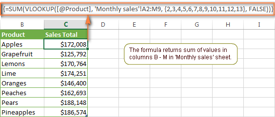
Tip. You may be curious why the formula displays [@Product] as the lookup value in the screenshot above. This is because I converted my data to table (Insert tab > Table). I find it very convenient to work with fully-functional Excel tables and their structured references. For example, when you type a formula into one cell, Excel automatically copies it across the entire column and in this way saves you a few precious seconds :)
As you see, using the VLOOKUP and SUM functions in Excel is easy. However, this is not the ideal solution, especially if you are working with big tables. The point is that using array formulas may adversely affect the workbook's performance since each value in the array makes a separate call of the VLOOKUP function. So, the more values you have in the array and the more array formulas you have in your workbook, the slower Excel works.
You can bypass this problem by using a combination of the INDEX and MATCH functions instead of SUM and VLOOKUP, and I will show you a few formula examples in the next article.
Download this VLOOKUP and SUM sample
How to perform other calculations with Excel VLOOKUP function
A moment ago we discussed an example of how you can extract values from several columns in the lookup table and calculate the sum of those values. In the same fashion, you can perform other mathematical calculations with the results returned by the VLOOKUP function. Here are a few formula examples:
| Operation | Formula example | Description |
|---|---|---|
| Calculate average | {=AVERAGE(VLOOKUP(A2, 'Lookup Table'$A$2:$D$10, {2,3,4}, FALSE))} | The formula searches for the value of cell A2 in 'Lookup table' and calculates the average of values in columns B,C and D in the same row. |
| Find maximum value | {=MAX(VLOOKUP(A2, 'Lookup Table'$A$2:$D$10, {2,3,4}, FALSE))} | The formula searches for the value of cell A2 in 'Lookup table' and finds the max value in columns B,C and D in the same row. |
| Find minimum value | {=MIN(VLOOKUP(A2, 'Lookup Table'$A$2:$D$10, {2,3,4}, FALSE))} | The formula searches for the value of cell A2 in 'Lookup table' and finds the min value in columns B,C and D in the same row. |
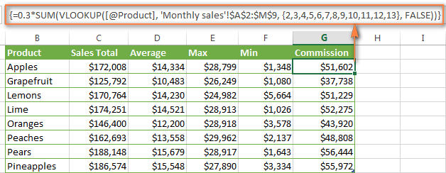
| Calculate % of sum | {=0.3*SUM(VLOOKUP(A2, 'Lookup Table'$A$2:$D$10, {2,3,4}, FALSE))} | The formula searches for the value of cell A2 in 'Lookup table', sums values in columns B,C and D in the same row, and then calculates 30% of the sum. |
Note. Since all of the above formulas are array formulas, remember to press Ctrl+Shift+Enter to enter them correctly in a cell.
If we add the above formulas to the 'Summary Sales' table from the previous example, the result will look similar to this:
Download this VLOOKUP calculations sample
LOOKUP AND SUM - look up in array and sum matching values
In case your lookup parameter is an array rather than a single value, the VLOOKUP function is of no avail because it cannot look up in data arrays. In this case, you can use Excel's LOOKUP function that is analogues to VLOOKUP but works with arrays as well as with individual values.
Let's consider the following example, so that you can better understand what I'm talking about. Suppose, you have a table that lists customer names, purchased products and quantity (Main table). You also have a second table containing the product prices (Lookup table). Your task is to make a formula that finds the total of all orders made by a given customer.
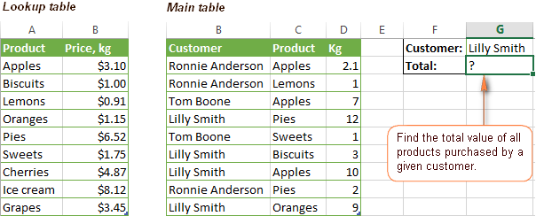
As you remember, you cannot utilize the Excel VLOOKUP function since you have multiple instances of the lookup value (array of data). Instead, you use a combination of SUM and LOOKUP functions like this:
=SUM(LOOKUP($C$2:$C$10,'Lookup table'!$A$2:$A$16,'Lookup table'!$B$2:$B$16)*$D$2:$D$10*($B$2:$B$10=$G$1))
Since this is an array formula, remember to press Ctrl + Shift + Enter to complete it.
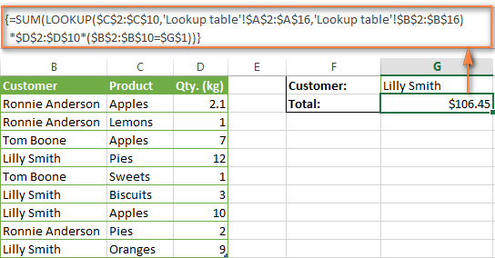
And now, let's analyses the formula's ingredients so that you understand how each of the functions works and can to tweak it for your own data.
We'll put aside the SUM function for a while, because its purpose is obvious, and focus on the 3 components that are multiplied:
LOOKUP($C$2:$C$10,'Lookup table'!$A$2:$A$16,'Lookup table'!$B$2:$B$16)This LOOKUP function looks up the goods listed in column C in the main table, and returns the corresponding price from column B in the lookup table.
$D$2:$D$10This component returns quantity of each product purchased by each customer, which is listed in column D in the main table. Multiplied by the price, which is returned by the LOOKUP function above, it gives you the cost of each purchased product.
$B$2:$B$10=$G$1This formula compares the customers' names in column B with the name in cell G1. If a match is found, it returns "1", otherwise "0". You use it simply to "cut off" customers' names other than the name in cell G1, since all of us know that any number multiplied by zero is zero.
Because our formula is an array formula it iterates the process described above for each value in the lookup array. And finally, the SUM function sums the products of all multiplications. Nothing difficult at all, it is?
Note. For the LOOKUP formula to work correctly you need to sort the lookup column in your Lookup table in ascending order (from A to Z). If sorting is not acceptable on your data, check out an awesome SUM / TRANSPOSE formula suggested by Leo.
Download this LOOKUP and SUM sample
VLOOKUP and SUMIF - look up & sum values with criteria
Excel's SUMIF function is similar to SUM we've just discussed in the way that it also sums values. The difference is that the SUMIF function sums only those values that meet the criteria you specify. For example, the simplest SUMIF formula =SUMIF(A2:A10,">10") adds the values in cells A2 to A10 that are larger than 10.
This is very easy, right? And now let's consider a bit more complex scenario. Suppose you have a table that lists the sales persons' names and ID numbers (Lookup_table). You have another table that contains the same IDs and associated sales figures (Main_table). Your task is to find the total of sales made by a given person by their ID. At that, there are 2 complicating factors:
- The mail table contains multiple entries for the same ID in a random order.
- You cannot add the "Sales person names" column to the main table.
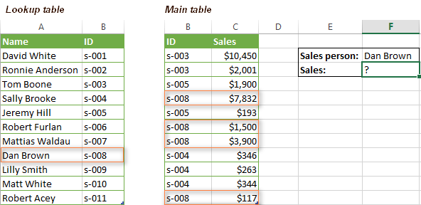
And now, let's make a formula that, firstly, finds all sales made by a given person, and secondly, sums the found values.
Before we start on the formula, let me remind you the syntax of the SUMIF function:
range- this parameter is self-explanatory, simply a range of cells that you want to evaluate by the specified criteria.criteria- the condition that tells the formula what values to sum. It can be supplied in the form of a number, cell reference, expression, or another Excel function.sum_range- this parameter is optional, but very important to us. It defines the range where the corresponding cells' values shall be added. If omitted, Excel sums the values of cells that are specified in the range argument (1st parameter).
Keeping the above info in mind, let's define the 3 parameters for our SUMIF function. As you remember, we want to sum all the sales made by a given person whose name is entered in cell F2 in the main table (please see the image above).
- Range - since we are searching by sales person ID, the range parameter for our SUMIF function is column B in the main table. So, you can enter the range B:B, or if you convert you data to a table, you can use the column's name instead:
Main_table[ID] - Criteria - because we have sales persons' names in another table (lookup table), we have to use the VLOOKUP formula to find the ID corresponding to a given person. The person's name is written in cell F2 in the main table, so we look it up using this formula:
VLOOKUP($F$2,Lookup_table,2,FALSE)Of course, you could enter the name in the lookup criteria of your VLOOKUP function, but using an absolute cell reference is a better approach because this creates a universal formula that works for any name input in a given cell.
- Sum range - this is the easiest part. Since our sales numbers are in column C named "Sales", we simply put
Main_table[Sales].Now, all you need is to assemble the formula's parts and your SUMIF + VLOOKUP formula is ready:
=SUMIF(Main_table[ID], VLOOKUP($F$2, Lookup_table, 2, FALSE), Main_table[Sales])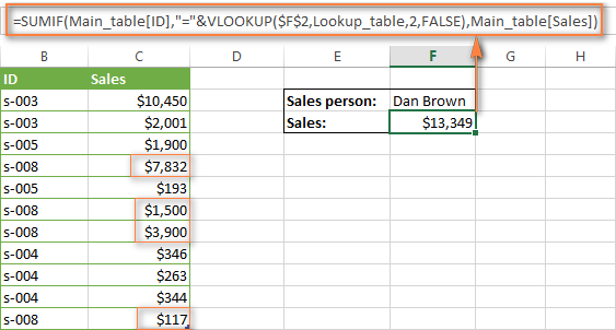
Download this VLOOKUP and SUMIF sample
Formula-free way to do vlookup in Excel
Finally, let me introduce you to the tool that can look up, match and merge your tables without any functions or formulas. The Merge Tables tool included with our Ultimate Suite for Excel was designed and develop as a time-saving and easy-to-use alternative to Excel's VLOOKUP and LOOKUP functions, and it can be very helpful both to beginners and advanced users.
Instead of figuring out formulas, you simply specify your main and lookup tables, define a common column or columns, and tell the wizard what data you want to fetch.
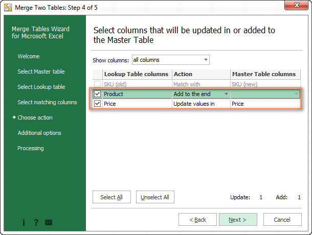
Then you allow the wizard a few seconds to look up, match and deliver you the results. If you think this add-in may prove helpful in your work, you are most welcome to download a trial version by using the below link.
Available downloads
VLOOKUP with SUM and SUMIF - formula examples (.xlsx file)
Ultimate Suite - trial version (.exe file)
 by
by
423 comments
I am trying to perform a vlookup of order numbers where I have a couple of duplicates which I want to sum into one number in my final table. I have tried playing around with
=IF(COUNTIF($P4:$V2598,$E4)>1, "Multiple results" ,VLOOKUP($E4,$P$4:$V$2598,6,FALSE))
But all I can do is print a message rather than displaying the result of my addition. Any ideas?
Hi everyone how can i consolidate the multiple duplicates with different values I need to sort out with the following ex below: I need the output that sums the total male > total female and total unkown under sample 1
list gender value
sample1 male 2
sample1 female 3
sample1 unknown 4
sample1 male 2
sample1 female 3
sample1 unknown 4
sample2 male 5
sample2 female 6
sample2 unknown 7
Glenn:
Where your sample data is organized like this:
Sample is in A30:A42, Gender is in B30:B42 and Value is in C30:C42 enter this formula in an empty cell:
=SUMIFS(C31:C42,A31:A42,"=Sample1",B31:B42,"=Male")
Hello,
I am currently trying to Sum number on a sheet (SHEET 1) within my workbook. On the same row of the amount that I want to sum is a specific description to that amount.
I am trying to SUMIF this amount to a different sheet (SHEET 2) corresponding to the matching description on the row from the other sheet (SHEET 1).
The amount varies by each entry. The matching descriptions will also vary.
I am trying to do this by keeping my filters and avoiding making tables for my data
I have Dates as column headers in a sheet. In another sheet I have to input date and I want a formula to search the relevant column on the basis of date input and sum the entries using a criteria on another colum simultaneously.
Hi,
Please, I will so much appreciate if you could help explain the use of the "Info!" excel function works in the below formula:
=VLOOKUP(P6,Info!C:I,7,0)
Many thanks.
It's not an Excel function, it's the sheet where the data is located.
Hi Sir/Mdm, I'm using =SUM(VLOOKUP(B2,A6:U105,MATCH(D2,A4:U4,0),0))"
to find a certain cell value. However, I need to sum up the values of the cells from B2 value till B3 Value. How should I do it?
Eg.
B2 = 1950
B3 = 1975
D2 = Metal
I need to enter value into Cell B2, B3 and D2. With the details entered, I need to sum up the value from "value of Row B2" to "value of Row B3" for the column of "value of Column D2".
Dear Sir,
Please give me suggestion/help for stock inventory sheet
Name of contractor Apple Banana Etc
Ram 2 5 4
Shyam 4 3 5
Hari 3 2 1
Ram 5 6 6
Hari 2 3 5
Saral 4 4 3
Ram 2 5 4
Shyam 4 3 5
Hari 3 2 1
Ram 5 6 6
Hari 2 3 5
Saral 4 4 3
I want to Total Issue to
"Ram"
Apple
Banana
Etc
Which formula's tell me sir.
Hi
I am trying to add total quantity sold by Name and ID same person.
=SUMIF('Q-1'!$B$4:$B$137,B4,'Q-1'!$K$4:$K$137)+SUMIF('Q-2'!$B$4:$B$137,B4,'Q-2'!$K$4:$K$137)+SUMIF('Q-3'!$B$4:$B$137,B4,'Q-3'!$K$4:$K$137)+SUMIF('Q-4'!$B$4:$B$137,B4,'Q-4'!$K$4:$K$137)
How can i short this formula with same answer?
i want to do total of 4 different sheets vlookup value.
Thanks
anybody help me please?
i have data below…
table1:
==========
ITEM | TYPE
==========
a1 | Cash
a2 | Cash
b1 | AP
c1 | AR
table2
=============
ITEM | AMOUNT
=============
a1 | 100
b1 |-100
a2 | 50
a1 | 40
b1 |-90
c1 | 200
result:
=============
TYPE | AMOUNT
=============
Cash | 190 (sumif?)
AP |-190 (sumif?)
AR | 200 (sumif?)
how do I populate a 'sumif' formula in the result table?
thanks & regards
i have used simple sumif formula and it works
as i have a table of values in one column (range 2) and criteria (range1) two and two cells out side as one for selecting the listed criteria and one for result on same sheet and applied the formula =sumif(range1, criteria, range2) in the cell where i expect the result.
thanks
Thank you very much for sharing.
how to use iferror and vlookup in excel for counting
Item Code Item Description
A1 Processors
A2 Printers
A3 Motherboards
This sample is belong to sheet1
Item Code Item Description
A1 vlookup formula pls!
This sample is belong to sheet2
what is the exact formula for the "item description" column in sheet number2, if I enter A1 on the "item code" column? the Processor should be the output.
Hello,
If I understand your task correctly, please try the following formula:
=VLOOKUP(A2,sheet1!$A$2:$B$4,2)
Hope this will help.
Item Code Item Description Item Code Item Description
A1 Processors A1 vlookup formula pls.
A2 Printers
A3 Motherboards
This sample is belong to sheet1 This sample is belong to sheet2
what is the exact formula for the "item description" column in sheet number2, if I enter A1 on the "item code" column the Processor should be the output.
I am looking to look up a product and calculate how much of it will be used.
I have Thousands of rows and 25+ collums
For example
MAIN BREAKDOWN
One & Half brick Walls
Bricks 10000
Cement 100
Building Sand 1000
One Brick Walls
Bricks 12000
Cement 120
Building Sand 1200
Half Brick Walls
Bricks 2500
Cement 15
Building Sand 15
Half Brick Walls
Bricks 2500
Cement 15
Building Sand 15
Half Brick Walls
Bricks 2500
Cement 15
Building Sand 15
BILL OF QUANTITIES (Seperate Sheet)
Bricks Sum of all Bricks
Cement Sum of all Cement
Building Sand Sum of all Building Sand
I need to add all of those up with out individually summing each one
There are over 200 rows that mention bricks
and we continually add in at various points of the sheet.
PLEASE HELP!
Hello,
For me to understand the problem better, please send me a small sample workbook with your source data and the result you expect to get to support@ablebits.com. Please don't worry if you have confidential information there, we never disclose the data we get from our customers and delete it as soon as the problem is resolved.
Please also don't forget to include the link to this comment into your email.
I'll look into your task and try to help.
in MS excel If there are three columns A, B and C, I need to get their sums to a new sheet which ones heading comes as Column B details Look up one as column A, need to create formula to get sum for column C.
in MS excel If there are three columns A, B and C, I need to get their sums to a new sheet which ones heading comes as Column B details Look up one as column A, need to create formula to get sum for column C.
A 10 25
A 8 30
B 5 45
A 10 30
10 8 5
A 55(Formula for this Number)
Hello,
I need to do almost exactly what you describe Under LOOKUP AND SUM - look up in array and sum matching values. However, while my lookup table is in fact vertical, my main table is horizontal. Hence, the formula you provide: {=SUM(LOOKUP($C$2:$C$10,'Lookup table'!$A$2:$A$16,'Lookup table'!$B$2:$B$16)*$D$2:$D$10*($B$2:$B$10=$G$1))}, does not work.
Any ideas?
Thanks!
I want to lookup the 593027761 value in Sheet 1 and sum of all the values in
Sheet 2 for lookup value in Sheet 1
Workbook 1
593027761
Workbook 2
593027761 100
593027761 200
593027761 600
593027761 5485
593027761 8784
593027761 2544
593027761 4898
593027761 544
593027761 54887
593027761 216564
593027761 5487
593027761 54656
593027761 553
593027761 221
Hi, Dharampal,
please a closer look at this point of the article above. It contains the example of the formula you need to create to solve your task.
Hope this helps.
hi
i need a function for the mentioned query
NAME SEGMENT TARGET
A R 2
A R 3
A R 2
B R 3
B BB 4
B R 2
A BB 1
A R 3
NAME A
NAME WISE TOTAL :
NAME WISE SEGMENT TOTAL :
Please suggest NAME WISE TOTAL Required and NAME with SEGMENT wise total required.
It is very very helpful for me.
i need to find name with address and amount and also date wise
main sheet is PT NAME with amount and date and ADDRESS DATA is second sheet with address and third sheet is required sheet with VLOOKUP FORMULA but i am not co relate with amount and date kindly help me for solving the problem.
I want to apply vlookup formula in excel sheet having pt. name and address and also i having data only pt. name how can match pt name with colour code?
I want to apply vlookup (or any) formula in excel sheet having pt. name and address and also i having data only pt. name how can match pt name with colour code?
09/11 10:18: Mast Devesh Aahuja Mast DEVESH AAHUJA Mast DEVESH AAHUJA 4 Y Dr. Asim Negi 44 tilak path khargone
13/12 12:48: Mast Dhananjay Magwani Mast DEVESH AAHUJA Mast DHANANJAY MAGWANI 15 Y Dr. Jitendra Pindoriya gram kampel teh. kampel
19/10 17:03: Mast Divyanshu Prajapat Mast DHANANJAY MAGWANI #N/A 45 Y Dr. Jitendra Thakur gram fangti teh. hatpipliya
12/10 20:55: Mast Gajendra Yadav Mast DHANANJAY MAGWANI #N/A 13 Y Dr. M.K Sharma gram mogawa teh. maheshwar
kindly help me.
Dear Svetlana Cheusheva,
Can I sent an excel Sheet with data to make Formula to calculating
the Data with criteria
regards
Hello Svetlana,
I'm looking to get the MAXIMUM of the multiple LOOKUP VALUES which are scattered and which are in different worksheets.
I tried with vlookup and index / match but could not do.
Example:
The answer when I try to vlookup for A0600 should be 1700 and not 1692 from the two lines given below:
A0600 23099090 XXXX 1692.00
A0600 23099090 XXXX 1700.00
Thank you so much in advance for your help!
Thiyagu.
I need some help. I have several tabs in an excel file with amounts per person (i.e. John $35, Kathy $40). Each person has a separate identifier (ID). I need to add all of John's amounts into one spreadsheet, all of Kathy's, etc. John may be in tab 1 and on tab 2 but not on tab 3. I think I need to use some vlookup combined with a sum but I can't figure out what to use. Can you please help me?
Thank you!
Country 2011 2012 2013 2014 2015
Japan 1653 1232 5319 9230 7647
Ukraine 5582 7685 7706 3723 6181
Japan 7330 5872 6723 6133 3228
Poland 4063 4337 4916 7608 4451
Germany 2330 3906 4673 1276 1592
Ukraine 7396 1752 8262 9823 9164
Germany 6690 5303 5155 4422 7661
Poland 1170 5878 6089 2398 3338
This is the date, now, for example, I want to use sumifs formula to calculate the sum of sales for Japan after 2012. Can you help? I tried the formula "=SUMIFS(B2:F9;A2:A9;G3;B1:F1;">"&G4)" but it did not work.
Hi,
Anyone can help for the formula of sumif. i got a total sum figure like 206.61.
Can the sumif formula find out from the column which of the value add on together is equal to 206.61.
Thank you.
Hi,
I was trying to make customers outstanding in 30-60 , 60-90 days old ,
i have the following sheet (With Formula),
A b c d e f
Name , Invoice date, Invoice No, Invoice amt , Balance, Due days
PICO 11/05/2017 653 3000.00 3000.00 75
I want to vie as below
a b
30-60 days, 60-90 days
3000.00
Can you help??/
HAVE SHEET CONTAINING EMPLOYEEID, GENDER, AGE, NO OF CHILDREN ETC.
ANOTHER SHEET CONTAINS EMPLOYEE ID,SALARY, LOANS ANY OTHER SIMILAR COLUMNS.
IN THE THE SECOND SHEET I WANT THE SUM OF SALARIES OF EMPLOYEES WHOSE AGE IS ,SAY 45,. I DONT WANT TO IMPORT THE AGE FROM SHEET1 USING LOOKUP AND THEN APPLYING SUMIF.
PLEASE SUGGEST ANY FORMULA SYNTAX WHICH WILL CHECK THE CRITERIA AN RETURN THE SUM OF SALARIES OF SUCH PEOPLE WHOSE AGE IS 45.
Sorry hit enter too quickly here is the example
Column A Column B Total
a 10 50
b 20
c 10
b 10
c 10
a 20
What i want is a function that will look at column a and add only the values in column b that are coded as b,c ie 50. Therefore if my next entries 3 entries are coded a and my fourth entry is code b with a value of 10 the function should ignore the ones coded a and add 10 to the total to get 60.
i hope you can help.
Thanks
I have a table that i populate every day. I want to calculate the total number of articles that are added to the previous day but only the ones that have a specific code. See example
Hi Svetlana
In below table array I need to sum quantity of repetitive items (same coded in column A)so they appear in new column as sampled below.
Could you please advise.
Many thanks
Pavel
A B C D
10052160 252.00 Pound 262.00
10052160 10.00 Pound 0.00
10072070 187.66 Pound 187.66
10072081 321.64 Pound 321.64
10072089 643.35 Pound 643.35
10072100 41.00 Can 41.00
10072111 30.64 Pound 30.64
10072130 40.51 Pound 40.51
10072170 243.68 Pound 243.68
10072175 216.76 Kg 385.40
10072175 73.65 Kg 0.00
10072175 209.74 Pound 0.00
i want to search out particular employees detail from the bulk employee list record....it is difficulty to find out manually search regarding the employees ...that's why plz send me the logical formula how it iz possible to find out through excel easily ......
Pricing Table Dilivery Table
No of Units Price/Unit Method R/Unit
1 70 Air 3
10 60 Rail 2.5
100 50 Road 2
200 40 Ship 1
500 30 Truck 1.5
1000 20
Sales Table
Deliver Method Units Sold Total Cost Unit Delivery
Air 25
Air 260
Rail 12
Rail 125
Road 150
Road 230
Ship 2
Ship 679
Truck 580
Truck 1010
Can You Please Assist me To Answer this Question
"The Pricing Table is placed in Columns A and B respectively while the Delivery Table is placed in Columns D and E of the Excel sheet. The Sales Table has 7 columns in Columns A, B, C, D, E, F and G respectively.
Exercise 1
What will be the “Total Cost” of products purchased for each delivery method, having been given the number of Units Sold in column B of the Sales Table? Using the LOOKUP Function tool in Excel 2013/365, write a formula in the TOTAL COST column (C12:C21) on the Sales Table to determine the Total Cost of products purchased in Rand. Thank you
Hi
was this question answered?
Hi
Please help me I have a spreadsheet with total columns for each customer, I need to put totals for each customer at the bottom and the totals must be the total paid invoices that I have formulated or for paid invoices. as I put invoice the total must appear
Pls help me.
there four colums
Date party Bags Status
02-Jan Raja 15 Lifted
02-Jan Prem 05 Lifted
03-Jan Raja 105 Process
Now i want a formula that how many bags lifted on 02-Jan ?/
HI
i have used if function and all the results of that function is a number, at the end i want to make the sum of all these results how to make that as the sum function wont make it as the result is not shown as a number
thanks
I have 20 codes in sheet 1 and need to sum up the total sum given on each codes from sheet 2. Can you help me come up the formula?
Ex.
Sheet 1:
CODE - TOTAL QTY
ABC1 - 2212
ABC2 - 271
ABC3 - 486
ABC4 - 111
Sheet 2:
Store1:
Code - Size Total Qty
ABC1 - 50in 500
ABC1 - 20in 604
ABC1 - 45in 332
ABC2- 64in 122
ABC2- 220in 123
ABC3- 123in 443
ABC4- 14in 443
ABC4- 122in 111
Store2:
Code - Size Total Qty
ABC1 - 50in 222
ABC1 - 20in 223
ABC1 - 45in 331
ABC2- 64in 15
ABC2- 220in 11
ABC3- 123in 43
Appreciate your advise for this formula
Hi Svetlana,
Could you please help me with my table. I have the below database with more than 680 rows of information. There are positive and negative values in the column, the total sum of which is zero. How do I build the formula to exclude all these matching values from the column?
Many thanks in advance for your help!
Kind regards
Hi, Viorica,
what do you understand by "matching values"? Those that are completely identical? Or maybe those of the same number but with different signs (positives/negatives)?
For now we can assume that if you have 0 as a result, it means that every positive value has a corresponding negative value. If you need to sum only positive ones, then:
=SUMIF(A1:J12, ">0")
For negatives only
=SUMIF(A1:J12, "<0")
If this won't solve your task, let us know more details.
Hello sir,
Could you help me I want to make my table. When I use SUMIF it just Sum for whole column only. I want to sum at concern code no. row and column. How can I sum code 100 in total by using SUMif or vlookup or hlookup or arry.
Code Job 1 job 2 job 3
100 $30
101 $50
103 $15
101 20
200 $10
103 $11
Best regards,
Ying Kham
Hello Svetlana,
I couldn't follow ur guide, could you pls help me guide to write one formula, forexample.
All my data in sheet2 and on sheet1 i have summary table that for specific ID of person i want summ all data from sheet2. how to do?
Hello,
I have a spreadsheet with different tabs. I want to figure out how to count how many sales of a particular product (9 products), was sold by each salesperson (150 sales people. In addition I want to figure out how much $ those sales produced by each salesperson. Theis data is housed on a tab called March 3 Data.
Please help.
Thank you
D
Hi.
I have an excel file with 30 tabs each with a range of financial data covering a 1yr period. I would like to, on a separate tab within the same file, create a formula which searches for the MAX and MIN value for each of those ranges of data, referencing (I suppose) two date cells which represent the range I am looking to search within. In other words, today, I would like to search for the MAX value during the last month on all of those tabs. And then, in a week, I would like to be able to adjust the search to again find the updated MAX value for the last month (ie, with the last data point being one week later). Can I do this? If so, how? Thanks, Kim
Hi,
Have a question regarding sum + vlookup. In your example, you made the col_index_num an array by using {2,3,4,5...}. Is there a way to make this dynamic by referencing a value in a cell? For example, I input a value into cell V1=2 and I would like it to sum over 12 columns i.e. V1 to V1+12. The array wont let me do {V1:V1+12}. Any help is appreciated.
Thanks
Praveen
across rows in the same column
I am trying to something very simple and cannot figure out how to do it by reading your examples. Let me explain. I have two spreadsheets where I am looking up the value in one an comparing it to the value in the other and where there is a match, returning the value in the corresponding column number =iferror(vlookup(B6,DetailDate!$D$59292:$BQ$59291,31,),0)
This returns the first value of the row that matches. The problem is that there are multiple rows that match and I need to sum them together before returning the value. What would the formula be?
The example sum(vlookup)you provided adds values across columns. I need to add them across rows.
I need to add the values in the same column but in multiple rows.
I tried to create an array for the one column (top to bottom) but it returns a 0 value.
Beautifully written and clear guide, thanks Svetlana!
I need some assistance with sumarising some detail information from the following sheet:
Category; Trx Date; VOLUME
In this sheet I have multiple categories that gets repeated on numerous Trx Dates.
I need to sumarise this information into a sheet that looks like this:
Trx Date 1 Trx Date2 Trx Date3
Category 1
Category 2
Category 3
Can someone please help me with the formula to achieve this.
Thanks