In this tutorial, you will find a handful of advanced formula examples that demonstrate how to use Excel's VLOOKUP and SUM or SUMIF functions to look up and sum values based on one or several criteria.
Are you trying to create a summary file in Excel that will identify all instances of one particular value, and then sum other values that are associated with those instances? Or, do you need to find all values in an array that meet the condition you specify and then sum the related values from another worksheet? Or maybe you are faced with a more concrete challenge, like looking through a table of your company invoices, identifying all invoices of a particular vendor, and then summing all the invoice values?
The tasks may vary, but the essence is the same - you want to look up and sum values with one or several criteria in Excel. What kind of values? Any numeric values. What sort of criteria? Any : ) Starting from a number or reference to a cell containing the right value, and ending with logical operators and results returned by Excel formulas.
So, does Microsoft Excel have any functionality that can help with the above tasks? Of course, it does! You can work out a solution by combining Excel's VLOOKUP or LOOKUP with SUM or SUMIF functions. The formula examples that follow below will help you understand how these Excel functions work and how to apply them to real data.
Please note, these are advanced examples that imply you are familiar with the general principles and syntax of the VLOOKUP function. If not, the first part of our VLOOKUP tutorial for beginners is certainly worth your attention - Excel VLOOKUP syntax and general usages.
Excel VLOOKUP and SUM - find the sum of matching values
If you work with numerical data in Excel, quite often you have not just to extract associated values from another table but also sum numbers in several columns or rows. To do this, you can use a combination of the SUM and VLOOKUP functions as demonstrated below.
Source data:
Suppose, you have a product list with sales figures for several months, a column per each month. The source data is on the sheet named Monthly Sales:

Now, you want to make a summary table with the total sales for each product.
The solution is to use an array in the 3rd parameter (col_index_num) of the Excel VLOOKUP function. Here is a generic formula:
As you see, we use an array constant in the third argument to perform several lookups within the same VLOOKUP formula in order to get the sum of values in columns 2,3 and 4.
And now, let's adjust this combination of VLOOKUP and SUM functions for our data to find the total of sales in columns B - M in the above table:
=SUM(VLOOKUP(B2, 'Monthly sales'! $A$2:$M$9, {2,3,4,5,6,7,8,9,10,11,12,13}, FALSE))
Important! Since you are building an array formula, be sure to hit Ctrl + Shift + Enter instead of a simple Enter keystroke when you finished typing. When you do this, Microsoft Excel encloses your formula in curly braces like this:
{=SUM(VLOOKUP(B2, 'Monthly sales'!$A$2:$M$9, {2,3,4,5,6,7,8,9,10,11,12,13}, FALSE))}
If you press the Enter key as usual, only the first value in the array will get processed, which will produce incorrect results.
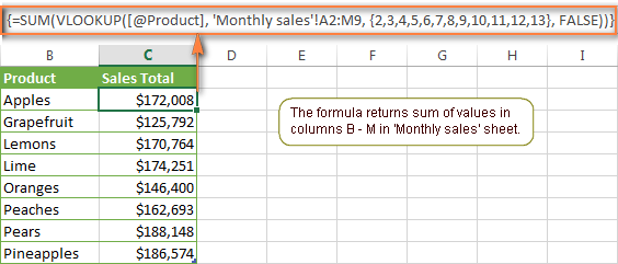
Tip. You may be curious why the formula displays [@Product] as the lookup value in the screenshot above. This is because I converted my data to table (Insert tab > Table). I find it very convenient to work with fully-functional Excel tables and their structured references. For example, when you type a formula into one cell, Excel automatically copies it across the entire column and in this way saves you a few precious seconds :)
As you see, using the VLOOKUP and SUM functions in Excel is easy. However, this is not the ideal solution, especially if you are working with big tables. The point is that using array formulas may adversely affect the workbook's performance since each value in the array makes a separate call of the VLOOKUP function. So, the more values you have in the array and the more array formulas you have in your workbook, the slower Excel works.
You can bypass this problem by using a combination of the INDEX and MATCH functions instead of SUM and VLOOKUP, and I will show you a few formula examples in the next article.
Download this VLOOKUP and SUM sample
How to perform other calculations with Excel VLOOKUP function
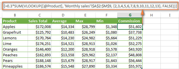
A moment ago we discussed an example of how you can extract values from several columns in the lookup table and calculate the sum of those values. In the same fashion, you can perform other mathematical calculations with the results returned by the VLOOKUP function. Here are a few formula examples:
| Operation | Formula example | Description |
|---|---|---|
| Calculate average | {=AVERAGE(VLOOKUP(A2, 'Lookup Table'$A$2:$D$10, {2,3,4}, FALSE))} | The formula searches for the value of cell A2 in 'Lookup table' and calculates the average of values in columns B,C and D in the same row. |
| Find maximum value | {=MAX(VLOOKUP(A2, 'Lookup Table'$A$2:$D$10, {2,3,4}, FALSE))} | The formula searches for the value of cell A2 in 'Lookup table' and finds the max value in columns B,C and D in the same row. |
| Find minimum value | {=MIN(VLOOKUP(A2, 'Lookup Table'$A$2:$D$10, {2,3,4}, FALSE))} | The formula searches for the value of cell A2 in 'Lookup table' and finds the min value in columns B,C and D in the same row. |
| Calculate % of sum | {=0.3*SUM(VLOOKUP(A2, 'Lookup Table'$A$2:$D$10, {2,3,4}, FALSE))} | The formula searches for the value of cell A2 in 'Lookup table', sums values in columns B,C and D in the same row, and then calculates 30% of the sum. |
Note. Since all of the above formulas are array formulas, remember to press Ctrl+Shift+Enter to enter them correctly in a cell.
If we add the above formulas to the 'Summary Sales' table from the previous example, the result will look similar to this:
Download this VLOOKUP calculations sample
LOOKUP AND SUM - look up in array and sum matching values
In case your lookup parameter is an array rather than a single value, the VLOOKUP function is of no avail because it cannot look up in data arrays. In this case, you can use Excel's LOOKUP function that is analogues to VLOOKUP but works with arrays as well as with individual values.
Let's consider the following example, so that you can better understand what I'm talking about. Suppose, you have a table that lists customer names, purchased products and quantity (Main table). You also have a second table containing the product prices (Lookup table). Your task is to make a formula that finds the total of all orders made by a given customer.
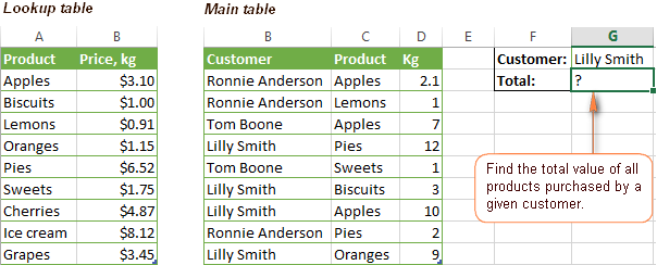
As you remember, you cannot utilize the Excel VLOOKUP function since you have multiple instances of the lookup value (array of data). Instead, you use a combination of SUM and LOOKUP functions like this:
=SUM(LOOKUP($C$2:$C$10,'Lookup table'!$A$2:$A$16,'Lookup table'!$B$2:$B$16)*$D$2:$D$10*($B$2:$B$10=$G$1))
Since this is an array formula, remember to press Ctrl + Shift + Enter to complete it.
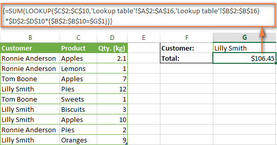
And now, let's analyses the formula's ingredients so that you understand how each of the functions works and can to tweak it for your own data.
We'll put aside the SUM function for a while, because its purpose is obvious, and focus on the 3 components that are multiplied:
LOOKUP($C$2:$C$10,'Lookup table'!$A$2:$A$16,'Lookup table'!$B$2:$B$16)This LOOKUP function looks up the goods listed in column C in the main table, and returns the corresponding price from column B in the lookup table.
$D$2:$D$10This component returns quantity of each product purchased by each customer, which is listed in column D in the main table. Multiplied by the price, which is returned by the LOOKUP function above, it gives you the cost of each purchased product.
$B$2:$B$10=$G$1This formula compares the customers' names in column B with the name in cell G1. If a match is found, it returns "1", otherwise "0". You use it simply to "cut off" customers' names other than the name in cell G1, since all of us know that any number multiplied by zero is zero.
Because our formula is an array formula it iterates the process described above for each value in the lookup array. And finally, the SUM function sums the products of all multiplications. Nothing difficult at all, it is?
Note. For the LOOKUP formula to work correctly you need to sort the lookup column in your Lookup table in ascending order (from A to Z). If sorting is not acceptable on your data, check out an awesome SUM / TRANSPOSE formula suggested by Leo.
Download this LOOKUP and SUM sample
VLOOKUP and SUMIF - look up & sum values with criteria
Excel's SUMIF function is similar to SUM we've just discussed in the way that it also sums values. The difference is that the SUMIF function sums only those values that meet the criteria you specify. For example, the simplest SUMIF formula =SUMIF(A2:A10,">10") adds the values in cells A2 to A10 that are larger than 10.
This is very easy, right? And now let's consider a bit more complex scenario. Suppose you have a table that lists the sales persons' names and ID numbers (Lookup_table). You have another table that contains the same IDs and associated sales figures (Main_table). Your task is to find the total of sales made by a given person by their ID. At that, there are 2 complicating factors:
- The mail table contains multiple entries for the same ID in a random order.
- You cannot add the "Sales person names" column to the main table.
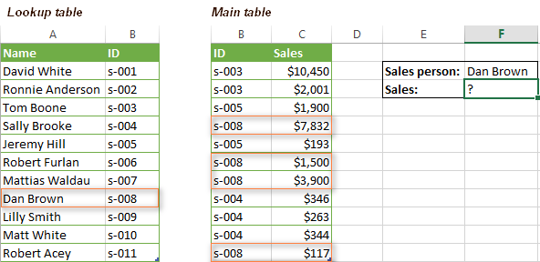
And now, let's make a formula that, firstly, finds all sales made by a given person, and secondly, sums the found values.
Before we start on the formula, let me remind you the syntax of the SUMIF function:
range- this parameter is self-explanatory, simply a range of cells that you want to evaluate by the specified criteria.criteria- the condition that tells the formula what values to sum. It can be supplied in the form of a number, cell reference, expression, or another Excel function.sum_range- this parameter is optional, but very important to us. It defines the range where the corresponding cells' values shall be added. If omitted, Excel sums the values of cells that are specified in the range argument (1st parameter).
Keeping the above info in mind, let's define the 3 parameters for our SUMIF function. As you remember, we want to sum all the sales made by a given person whose name is entered in cell F2 in the main table (please see the image above).
- Range - since we are searching by sales person ID, the range parameter for our SUMIF function is column B in the main table. So, you can enter the range B:B, or if you convert you data to a table, you can use the column's name instead:
Main_table[ID] - Criteria - because we have sales persons' names in another table (lookup table), we have to use the VLOOKUP formula to find the ID corresponding to a given person. The person's name is written in cell F2 in the main table, so we look it up using this formula:
VLOOKUP($F$2,Lookup_table,2,FALSE)Of course, you could enter the name in the lookup criteria of your VLOOKUP function, but using an absolute cell reference is a better approach because this creates a universal formula that works for any name input in a given cell.
- Sum range - this is the easiest part. Since our sales numbers are in column C named "Sales", we simply put
Main_table[Sales].Now, all you need is to assemble the formula's parts and your SUMIF + VLOOKUP formula is ready:
=SUMIF(Main_table[ID], VLOOKUP($F$2, Lookup_table, 2, FALSE), Main_table[Sales])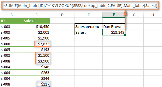
Download this VLOOKUP and SUMIF sample
Formula-free way to do vlookup in Excel
Finally, let me introduce you to the tool that can look up, match and merge your tables without any functions or formulas. The Merge Tables tool included with our Ultimate Suite for Excel was designed and develop as a time-saving and easy-to-use alternative to Excel's VLOOKUP and LOOKUP functions, and it can be very helpful both to beginners and advanced users.
Instead of figuring out formulas, you simply specify your main and lookup tables, define a common column or columns, and tell the wizard what data you want to fetch.
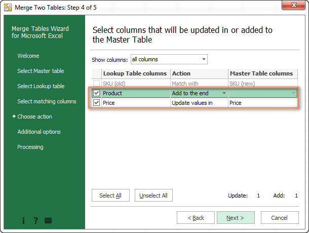
Then you allow the wizard a few seconds to look up, match and deliver you the results. If you think this add-in may prove helpful in your work, you are most welcome to download a trial version by using the below link.
Available downloads
VLOOKUP with SUM and SUMIF - formula examples (.xlsx file)
Ultimate Suite - trial version (.exe file)
 by
by
423 comments
I HAVE 2 SPREADSHEET AND I WANT INVOICE NO. FROM 2ND SHEET IN 1ST SHEET BUT CONDITION IS THAT ALL PRODUCT CODE DETAILS MATCH WITH 2ND SHEET PRODUCT CODE PLEASE HELP ME WHAT FORMULA I USE.
I have a spreadsheet that adds up daily usage of a material and subracts from the balance. It also adds that incoming inventory back in.
Example =(K3781+I3782)-(J3782)
Currently I manully enter the projected usage into this cell, this then gives me the projected balance.
Example =(K3781+I3782)-(J3782)-940-568
I would like to be able to export the information into another tab and excel calculate for me. The problem that I have is that multiple usage on the same date. I dont want to sum because I would like to associate the usage to a partiacular number. I can also have the same number on the same date that drives usage. Would it be possible submit an eample of what I am trying to explain?
hi,
am looking for a formula where I can average 7 values from 8 by taking the first 5 and choosing the best 2 from the remaining 3 values.
hi
I am getting close to the formula
i want to enter a serial number in Column B1:B23 page 1
then it matches serial number page 2 column A:1:a23
than data(written and date) from page 2 column b,c shows up in page 1 column c,d
i cant get it without error and both columns showing up
Hi, So I have a column A of name of people and their spending in a year in Column. I need to calculate how much each person spent by looking up the name so that if new entries are added the SUM automatically gets updated. Is their a way?
So close. The solution I used was SUMIFS which is similar but uses two columns to grab info from a third.
Thanks.
Does the Vlookup and Sum work with repeated values? for example if you had 2 columns with the name apples and want to sum both of the totals for both of the apple columns into one combined total. I am trying to generate a spreadsheet that will wind repeating cost codes and add the repeating cost codes for me. Please let me know how i can go about this!
Hi
As part of a larger problem I want to calculate the sum of top "n" values, where n will be user defined.
The sum will be calculated for an array,which has been calculated using several conditions using array formulas.
Eg: After all the conditional array formula, say I am getting an array as {0;23;45;0;0;10;1}
This array is dynamic based on the conditions provided. So, is there a way to find the sum of say first 3 or first 4 non zero numbers from this arrray ?
Thanks in advance
Thanks for the great article and I'm hope I'm not repeating a previous question...
When writing in the numbers of your array {2, 3, 4, 5, 6} and so on, is there a way to list an entire range of values at once? Say if you want to sum indexes 2 to 100. I noticed you mentioned the index function if I'm trying to sum over hundreds of columns for a given criteria. Should I not be using this array vlookup option for this case?
Happy to investigate another link if the answer is already out there. Pass it my way.
Thanks again for your clear explanations!
Ed
Hi all
Could you please tell me how in range of say some amounts, how to arrive at a particular sum amount. Suppose I have 50 Invoice amount due from a customer. I received a payment which includes 10-20 invoices. how can i know which amounts add to that particular cheque amount. Could you please give me the formula. Thanks
how to use sum and v lookup farmula from multiple rows
BANK 301370
BANK 736310
BANK 1473600
CONST. 100
CONST. 200
CONST. 200
CONST. 200
CONST. 200
CONST. 218
CONST. 300
CONST. 29000
CONST. 50000
CONST. 68800
FREIGHT 50
FREIGHT 200
FREIGHT 450
GENERAL 50
GENERAL 200
GENERAL 220
GENERAL 250
GENERAL 300
GENERAL 380
i want sprate total like summery
Hi, I hope someone can help. I would like to add up 2 sets of 2 columns with multiple codes for certain results.
For example/
Column A (company) consists of:#1 and #0
Column B (company) consists of:for #1 - A,B,C,D,Z
for #0 - F,G,H,I,J,K,L,M
Column D (contact) consists of: #0, #1 and #2
Column E (contact) consists of: for #0 - A, B
for #1 - C, D, E, F, G, J
for #2 - C,D,E,F,G,I,K,L,Z
Thanks in advance
Hello Dear,
i know sumif formula. But i don't no vlookup sum formula that means ID Value Total. for Example,
Sheet1,
ID Value
A1 100
B1 200
C1 300
A1 500
B1 300
C1 400
and i needed ID wise sum A1=100+500=600.
B1=200+300=500.
Please help me.
I have a spreadsheet for monthly/yearly overtime worked per job position at my company. People can also be charged time and a half or time and three quarters, depending on their schedule.
I need a way to search column b for job position and column c for type of schedule and if those equal PositionA ScheduleA to add column f's numbers all together in Cell Y. If PositionA Schedule B, add them together in Cell Z.
Is that too complicated for Excel?
Hello,
Is it possible to sum a row of numbers only if those numbers are from a formula? I am using a forecasting spreadsheet and any future figures are input manually by the budget managers as a 'guess'. However the actual spends for each month up until that point are found by using a VLOOKUP formula.
Basically I want to only sum the numbers if they are from the VLOOKUP formula.
Thank you for any help you can provide.
Hi All
I hope you are all well.
I don't know if this is going to be a bit of a stupid question, and I hope I make myself as understandable as possible. :)
Firstly, I am using Excel 2016 on Windows 10.
This is the scenario:
Book 1
- I have one Excel workbook with individual invoices for multiple customers. For example, the most important info:
Column A - Customer name (There are sometimes more than a few invoices for one customer)
Column B - Date
Column C - Invoice amount
Book 2
- I have another Excel workbook with the same as above, but they are credits relating to those invoices/customers:
Column A - Customer name (Same as above - more than a few lines for one customer, many different customers)
Column B - Date
Column C - Credit amount
Book 3
- The other Excel workbook is a consolidation of the above. I need to consolidate the above by customer, by month (working on November 2015 to October 2016 MTD). I considered doing a VLOOKUP by customer, but I don't know how to do a SUM VLOOKUP to add together all invoices for one customer in a date range from Book 1 onto Book 3, then the same for the credits from Book 2 to Book 3, so that I can calculate the difference.
I hope someone can assist me with this, and that I have made the question quite clear. :)
Thanks in advance!
How can I remove N/A
Sheet 1 Sheet2 Sheet 3 Sheet 4
As=(Vloopup)+(Vlookup)+(Vlookup)+(Vloopup) from different sheet, one sheet have no value(Like Sheet 4), but other sheet have value(Sheet 1,2,3) its showing N/A. If I use IF(ISERROR(Vlookup), then showing 0. But its not true.How can i solve this problem
Urgent
Hi,
I am trying to combine a SUMIFS and a VLOOKUP. My data set is big, and I run into problems when a name that used to be in the data is deleted from the data. That is why I want the forumla to lookup at the ID number of the person in my spreadsheet first, and then match it with their value in the data tab. Some people are in there twice, same ID but different two different values. I was a forumala that will match to the first and then match to the second.
Can someone help with this?
i have tried this with sumif(vlook up) but i dont get the esult and i cudnt find my error in formula
Hi
I am trying to do a sumif. The criteria are on two separate tabs. I want to sum if the attribute is "adjustable", but this attribute is on a separate tab so I have to do a vlookup to see if it is adjustable or not. Once something is adjustable, then it should be summed up. I've tried the following two formulae, and they don't seem to work:
=SUMIFS('LG dataset Subfund Method'!I$2:I$611,vlookup('LG dataset Subfund Method'!F2,'Attributes Matrix'!$A$2:$G$611,7,false),Adjustable)
and
=SUMIFS('LG dataset Subfund Method'!I$2:I$611,INDEX('Attributes Matrix'!$G$2:$G$611,MATCH('Attributes Matrix'!A2,'Attributes Matrix'!$A$2:$A$611,0)),Adjustable)
Basically I'm trying to create a logic that says sum up the cashflows on the LG tab only if the attribute attached to the plancode is Adjustable and this part is on the Attributes Matrix tab.
Hi.,,
May I Know How To Add Number with the Help of Vlook_Up..
For Ex:
Sharat
Fruits Numbers
Apple 190
Banana 111
Mango 503
Geeta
Mango 113
Banana 190
Apple 190
watermelon 190
Ram
Banana 128
Apple 147
watermelon 180
Mango 114
..
...
How i Can Add Like......
Fruits Total Items
Total Banana ?
Total Apple ?
Total Mango ?
Total watermelon ?
Hi, I have a worksheet with a matrix of names (6 columns of differing names in each rwo) and in another column I have either "Won" or "Lost".
I want to count the number of "Won"s for each person.
So I have a formula: =COUNTIFS(TMT!$F$2:$K$29,B4) which finds and counts all the times the person's name in B4 exists. This works OK.
But when I add another selection =COUNTIFS(TMT!$F$2:$N$29,B4,TMT!D:D,"=Won") I get an error "A value used in the formula is a wrong data type". However if I enter only the second selection on it's own I get no error.
Any ideas?
Dear Philip Morris just remove = of "=won" from =COUNTIFS(TMT!$F$2:$N$29,B4,TMT!D:D,"=Won")
Hi,
I have to find sum of sale qnty using vlookup
first sheet where purchase is
Code Qnty
NFSC 2
NFCC 5
NFDD 7
Other sheet where sale of the month is (date wise sale)
Code Qnty
NFSC 1
NFCC 1
NFDD 1
NFSC 1
NFDD 1
NFCC 1
Hi there,
Your tutorial is good but i'm struggling to adapt it to my situation and wondered if you could help?
I have a workbook for timesheets that contains 53 sheets, one for every week. Each sheet is formatted the same and shows the job number and job name in rows above one and other in the first column. These rows are then combined in the next column to show total hours worked, then the next columns represent the actual days of the week and hours worked per day.
I would like to have a summary table at the end of the workbook that tells me total hours worked in the year and total hours spent per job number. i've tried a variety of sum and look up combinations and nothing has worked yet.
any pointers you can make would be greatly appreciated.
Respected Able Bits Team;
Please give me merge tables wizard excel 2003 .xls format
Regards
Saurabh Sharma
Hi,
I have a fairly simple task that I just can't figure out a formula for it. I have a range of account # that I need to find and sum on one cell.
For example,
I need to sum account numbers 2001-2020. All accounts from 1000 to 3000 are listed in column B (in another tab within the same work book). Column C in that same tab has the account values that I need to sum.
I tried the SUM-LOOKUP combo but sorting in ascending order is not an option for me. What other formula can I use to get to my desired result?
I would really appreciate your help with this!
Hello Svetlana,
What you have shown is simply amazing and I sincerely appreciate the time and effort you have put. Thanks a lot!
I have a small query which I believe has no solution but would like your opinion on. So I am working on a case similar to SUMIF and VLOOKUP combination example above, but the difference is that my lookup array is spread across multiple worksheet and not just one main table. Any thoughts on how to resolve it? I was thinking using SUMIFS and VLOOKUP maybe, but not sure! :-(
Anky
How to calculate catagory wise cummilative value like
Mc. Qty
Duke120. 3
Duke 220. 4
Deke 330. 3
pulser 120. 5
Pulser 220. 7
Pulser 250. 8
Now what im want is cummilative value of duke and cummilative value of pulser different wise but on a same column.
when i create invoice ...then automatic stock credit or debit.,amount plus in customer account.,when enter part number then automatic fill part discription....i wish this formula
Good Day! What is the formula for the =Sum(Vlookup) For vertical addition of data?
Regards
Tlhogi
I have been struggling to fulfill my boss requirement but still unsuccessful. Maybe someone can help me with the quickest way.
I have a workfile with multiple sheets but each sheets uses the same format. Example:
Sheet 1.
Part Name: ABC
Type of Defects 1-May 2-May 3-May 4 May
Defects 1 10 100 50 60
Defects 2 12 50 20 30
Sheet 2 or 3 or 4 are the same as sheet 1 except
Part Names are different
I want to create a Summary page whereby I just need to key in the following criteria:
Part Name : XXXX ( just key in the part number )
Date Start : Select which start date
Date End : Select which end date
With this 2 criteria typed in, all the defects will automatically add up but still separated still into Defects 1 and Defects 2.
In other words, the left hand column will still have Defects 1 and Defects 2 and so on.
Can someone help me?
Hye,
I'm meeting trouble in doing sum of different vlookup values. I try explain my problem with an example given below:
| A |B |C |D |E |F
1| 02-01 |48 |22 |38 |54 |98
2| 03-01 |20 |105|111|50 |40
3| 03-02 |35 |40 |67 |66 |901
4| 03-03 |88 |50 |100|47 |200
In given above table I want to sum all values vertically in column F with reference to Column A but want to add only that values of which code in Column A start with 03.
Please guide me. You can mail reply on my mail ID if convenient. Thanks
i want lookup A3 value in range B3:B10 if cell value verify then result show with text and commas
one problem mostly i face when i update the advance of employee .the problem is . there are three column
column(A) column(B) column(C)
employee punch n. Advance
mohit 54 1500
mukesh 84 2500
rahul 90 2000
mohit 54 500
sabir 92 5000
is there any formula that add the amount that is double to a employee
by a formula in excel sheet when i prepare salary and adjust the advance .
Hi Svetlana,
I have a data in which first row contains date and other three rows contains their pageviews, visits. I need your help to merge date wise data in which i can the total visits pageviews and as well as visitors for all dates seperately this database contains 4700 rows.
Below are the example of data.
Looking forward for your reply.
Date Visitors Visits Page Views
1-Jan-08 110,318 143,414 165,477
1-Jan-08 111,056 144,372 166,583
1-Jan-08 112,961 146,850 169,442
1-Jan-08 110,977 144,271 166,466
1-Jan-08 110,561 143,730 165,842
1-Jan-08 105,094 136,622 157,641
1-Jan-08 112,742 146,565 169,113
1-Jan-08 108,948 141,632 163,422
1-Jan-08 110,211 143,274 165,316
1-Jan-08 107,731 140,050 161,596
2-Jan-08 107,917 140,292 161,876
2-Jan-08 109,908 142,880 164,862
2-Jan-08 105,705 137,417 158,558
2-Jan-08 106,791 138,829 160,187
Thanks,
Nandan
You can use Paviot Table. It will surely convenient for you.
Paviot Table can be added from Insert tab.
how can we solve it by only using vlookup....
Hi,
I have 12 columns and thousands of rows. On columns I have (Years-Months-Factories-a-b-c-d-e-f-volume-sales-price)..What I want to do is, I want to calculate total volume for each factory(4 factory) by months in each year..
Thx
hi,
I am using 2 sheets with daily sales in sheet1 and inventory in sheet2. I want to put sum formula in sheet2 so that it pick an item no and goes to sheet1, locates its occurrence and than calculate from values in corresponding columns. But the tricky part are, first, values are in 3 columns - sale(-), return(+) and stock delivery(+). Second, sale for same item will happen on multiple days, so all will be factored in and entered before the item in inventory list.
I have input an array formula with sum and vlookup in sheet 2. It gives value for only one column and one row.
Please help.
i need to calculate the average value for male and female students in class. but their title in different page and final mark in different page. need to do it using vlookup..
can i be able to do sum of the various values having base as sku code (ex:20001218 -1
in the same i have the other one to )
Hi,
I have a excle worksheet. in that there are every month salary detail in different month sheet. I want to get total of salary of the year in one sheet against his/her name. How to do it with Vlookup formula. Kindly suggest me.
Thanks...
Great Forum for learning! really appreciate Svetlana & Teams efforts. Thanks!
Hi
Require a help
I have a rows of values like this
5000
2000
7000
15161
5000
In another cell i have a value 25161
In the rows if i add some way i should be getting 25161 ( example 5000+15161+5000) will match my 25161,
Is there any formula to achieve this
what formula i need to use for below
sheet one - GL code, vendor name and Feb amount in column. One vendor has multiple GL codes
Sheet two - Same has above but amount is for JAN
I need to bring jan amount to sheet one next to feb amount to see the varience
since one vendor has multiple gl codes just vlookup formula is not working. What i need to do here
HI
I want to count the value in subgroup for example:
A
B
C
d
d
d
C
d
B
C
d
d
d
I want to know how many "d" are in the first "C" group
Or how many "d" are in the first "B" group
"Count "d" from current value to same value in column.
so tnx
Hi- I need help on following table to combine vlookup and sumif.
Table :
A -2
A 4
A -3
B -4
A -4
B 7
I need formula to calculate only for negative sum from column 2 and vlookup for column.
Results should be like this
A -9
B -4
Can you help to create formula for this?
Thanks, Rahul
sent me in my email i well do for you.
Dear Sir i have 3 sheets of diffrent subject having same table... and i want to find the result in one click... for example i want to find the result of pecentage on single cell by given roll number
Formula Required if in a cell contains 10 digit Pan Number AKRPD3915C if the 4th Letter P it should show as "Person" and if the 4th Letter C it show as "Company"
I need your help, I just want to one cell contain text in other cell list i think formula =ISNUMBER(FIND(E47,B3:B991)) in this E47 is my targeted cell
helo,
please I need your help.
is there any formula that spell a number or any currency ???
Appreciate your support
Hello hope that someone can help me? i need a formula that allows me to sum up the hours worked a day, the problem is it needs to be by name for example.
harry worked from 09:00 till 09:30
carlos from 10:00 till 10:30.
etc
how can i make excel add the worked hours behind carlos his name?
thank you
this is for a working schedule that sums up the worked hours as well.