This tutorial explains the difference between the SUMIF and SUMIFS functions in terms of their syntax and usage, and provides a number of formula examples to sum values with multiple AND / OR criteria in Excel 365, 2021, 2019, 2016, 2013, 2010, and lower.
As everyone knows, Microsoft Excel provides an array of functions to perform various calculations with data. A few articles ago, we explored COUNTIF and COUNTIFS, which are designed for counting cells based on a single condition and several conditions, respectively. Last week we covered Excel SUMIF that adds values meeting the specified criteria. Now it's time to go over the plural version of SUMIF - Excel SUMIFS that allows summing values by multiple criteria.
Those who are familiar with the SUMIF function might think that converting it to SUMIFS takes just an extra "S" and a few additional criteria. This would seem quite logical… but "logical" it's not always the case when dealing with Microsoft : )
Excel SUMIF function - syntax & usage
The SUMIF function is used to conditionally sum values based on a single criteria. We discussed the SUMIF syntax in detail in the previous article, and here's just a quick refresher.
- range - the range of cells to be evaluated by your criteria, required.
- criteria - the condition that must be met, required.
- sum_range - the cells to sum if the condition is met, optional.
As you see, the syntax of the Excel SUMIF function allows for one condition only. And still, we say that Excel SUMIF can be used to sum values with multiple criteria. How can that be? By adding the results of several SUMIF functions and by using SUMIF formulas with array criteria, as demonstrated in the examples that follow.
Excel SUMIFS function - syntax & usage
You use SUMIFS in Excel to find a conditional sum of values based on multiple criteria. The SUMIFS function was introduced in Excel 2007 and is available in all subsequent versions of Excel 2010, 2013, 2016, 2019, 2021, and Excel 365.
Compared to SUMIF, the SUMIFS syntax is a little bit more complex:
The first 3 arguments are mandatory, additional ranges and their associated criteria are optional.
sum_range- one or more cells to sum, required. This can be a single cell, a range of cells or a named range. Only cells with numbers are summed; blank and text values are ignored.criteria_range1- the first range to be evaluated by the associated criteria, required.criteria1- the first condition that must be met, required. You can supply the criteria in the form of a number, logical expression, cell reference, text or another Excel function. For example you can use criteria such as 10, ">=10", A1, "cherries" or TODAY().criteria_range2, criteria2, …- these are additional ranges and criteria associated with them, optional. You can use up to 127 range/criteria pairs in SUMIFS formulas.
Notes:
- For a SUMIFS formula to work correctly, all the criteria_range arguments must have the same dimension as sum_range, i.e. the same number of rows and columns.
- The SUMIFS function works with AND logic, meaning that a cell in the sum range is summed only if it meets all of the specified criteria, i.e. all the criteria are true for that cell.
Basic SUMIFS formula
And now, let's have a look at the Excel SUMIFS formula with two conditions. Suppose, you have a table listing the consignments of fruit from different suppliers. You have the fruit names in column A, suppliers' names in column B, and quantity in column C. What you want is to find out a sum of amounts relating to a given fruit and supplier, e.g. all apples supplied by Pete.
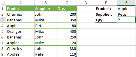
When you're learning something new, it's always a good idea to start with simple things. So, to begin with, let's define all the arguments for our SUMIFS formula:
- sum_range - C2:C9
- criteria_range1 - A2:A9
- criteria1 - "apples"
- criteria_range2 - B2:B9
- criteria2 - "Pete"
Now assemble the above parameters, and you will get the following SUMIFS formula:
=SUMIFS(C2:C9, A2:A9, "apples", B2:B9, "Pete")
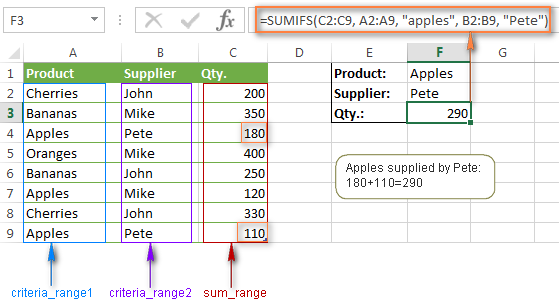
To refine the formula further, you can replace the text criteria "apples" and "Pete" with cell references. In this case, you won't have to change the formula to calculate the quantity of other fruit from a different supplier:
=SUMIFS(C2:C9, A2:A9, F1, B2:B9, F2)
Note. Both the SUMIF and SUMIFS functions are case-insensitive by nature. To get them to recognize the text case, please see Case-sensitive SUMIF and SUMIFS formula in Excel.
SUMIF vs. SUMIFS in Excel
Since the aim of this tutorial is to cover all possible ways to sum values by several conditions, we will discuss formula examples with both functions - Excel SUMIFS and SUMIF with multiple criteria. To use them correctly, you need to clearly understand what these two functions have in common and in what way they are different.
While the common part is clear (similar purpose and parameters), the differences are not so obvious, though very essential.
There are 4 major differences between SUMIF and SUMIFS:
- Number of conditions. SUMIF can evaluate just one condition at a time while SUMIFS can check for multiple criteria.
- Syntax. With SUMIF, the sum_range is the last and optional argument - if not defined, the values in the range argument are summed. With SUMIFS, sum_range is the first and required argument.
- Size of ranges. In SUMIF formulas, sum_range does not necessarily have to be of the same size and shape as range, as long as you have the top left cell right. In Excel SUMIFS, each criteria_range must contain the same number of rows and columns as the sum_range argument.
For example, SUMIF(A2:A9,F1,C2:C18) will return the correct result because the leftmost cell in the sum_range argument (C2) is right. So, Excel will make the correction automatically and include as many columns and rows in sum_range as there are in range.
A SUMIFS formula with unequally sized ranges will return a #VALUE! error.
- Availability. SUMIF is available in all Excel versions, from 365 through 2000. SUMIFS is available in Excel 2007 and higher.
Alright, enough strategy (i.e. theory), let's get into the tactics (i.e. formula examples : )
How to use SUMIFS in Excel - formula examples
A moment ago, we discussed a simple SUMIFS formula with two text criteria. In the same manner, you can use Excel SUMIFS with multiple criteria expressed by numbers, dates, logical expressions, and other Excel functions.
Example 1. Excel SUMIFS with comparison operators
In our fruit suppliers table, suppose, you want to sum all deliveries by Mike with Qty. 200 or more. To do this, you use the comparison operator "greater than or equal to" (>=) in criteria2 and get the following SUMIFS formula:
=SUMIFS(C2:C9,B2:B9,"Mike",C2:C9,">=200")
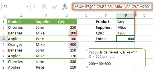
Note. Please pay attention that in Excel SUMIFS formulas, logical expressions with comparison operators should always be enclosed in double quotes ("").
We covered all possible comparison operators in detail when discussing Excel SUMIF function, the same operators can be used in SUMIFS criteria. For example, the following formula with return the sum of all values in cells C2:C9 that are greater than or equal to 200 and less than or equal to 300.
=SUMIFS(C2:C9, C2:C9,">=200", C2:C9,"<=300")
Example 2. Using Excel SUMIFS with dates
In case you want to sum values with multiple criteria based on the current date, use the TODAY() function in your SUMIFS criteria, as demonstrated below. The following formula sums values in column D if a corresponding date in column C falls within the last 7 days, including today:
=SUMIFS(D2:D10, C2:C10,">="&TODAY()-7, C2:C10,"<="&TODAY())
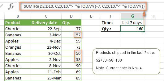
Note. When you use another Excel function together with a logical operator in the criteria, you have to use the ampersand (&) to concatenate a string, for example "<="&TODAY().
In a similar fashion, you can use the Excel SUMIF function to sum values in a given date range. For example, the following SUMIFS formula adds the values in cells C2:C9 if a date in column B falls between 1-Oct-2014 and 31-Oct-2014, inclusive.
=SUMIFS(C2:C9, B2:B9, ">=10/1/2014", B2:B9, "<=10/31/2014")
The same result can be achieved by calculating the difference of two SUMIF functions, as demonstrated in this example - How to use SUMIF to sum values in a given date range. However, Excel SUMIFS is much easier and more understandable, isn't it?
Example 3. Excel SUMIFS with blank and non-blank cells
When analyzing reports and other data, you may often need to sum values corresponding either to empty or non-empty cells.
| Criteria | Description | Formula Example | |
|---|---|---|---|
| Blank cells | "=" | Sum values corresponding to blank cells that contain absolutely nothing - no formula, no zero length string. | =SUMIFS(C2:C10, A2:A10, "=", B2:B10, "=")
Sum values in cells C2:C10 if the corresponding cells in columns A and B are absolutely empty. |
| "" | Sum values corresponding to "visually" blank cells including those that contain empty strings returned by some other Excel function (for example, cells with a formula like =""). | =SUMIFS(C2:C10, A2:A10, "", B2:B10, "")
Sum values in cells C2:C10 with the same conditions as the above formula, but includes empty strings. |
|
| Non-blank cells | "<>" | Sum values corresponding to non-empty cells, including zero length strings. | =SUMIFS(C2:C10, A2:A10, "<>", B2:B10, "<>")
Sum values in cells C2:C10 if the corresponding cells in columns A and B are not empty, including cells with empty strings. |
| SUM-SUMIF or SUM / LEN |
Sum values corresponding to non-empty cells, not including zero length strings. | =SUM(C2:C10) - SUMIFS(C2:C10, A2:A10, "", B2:B10, "")
=SUM((C2:C10) * (LEN(A2:A10)>0)*(LEN(B2:B10)>0)) Sum values in cells C2:C10 if the corresponding cells in columns A and B are not empty, cells with zero length strings are not included. |
And now, let's see how you can use a SUMIFS formula with "blank" and "non-blank" criteria on real data.
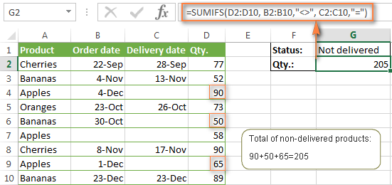
Suppose, you have an order date in column B, delivery date in column C and Qty. in column D. How do you find the total of products that have not been delivered yet? That is, you want to know the sum of values corresponding to non-empty cells in column B and empty cells in column C.
The solution is to use the SUMIFS formula with 2 criteria:
=SUMIFS(D2:D10, B2:B10,"<>", C2:C10,"=")
Using Excel SUMIF with multiple OR criteria
As noted in the beginning of this tutorial, the SUMIFS function is designed with AND logic. But what if you need to sum values with multiple OR criteria, i.e. when at least one of the conditions is met?
Example 1. SUMIF + SUMIF
The simplest solution is to sum the results returned by several SUMIF functions. For example, the following formula demonstrates how to find the total of products delivered by Mike and John:
=SUMIF(C2:C9,"Mike",D2:D9) + SUMIF(C2:C9,"John",D2:D9)
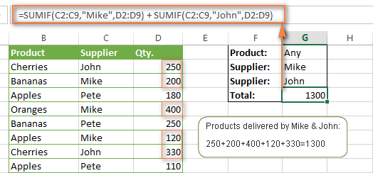
As you see, the first SUMIF function adds the quantities corresponding to "Mike", the other SUMIF function returns the amounts relating to "John" and then you add these 2 numbers.
Example 2. SUM & SUMIF with an array argument
The above solution is very simple and may get the job done quickly when there are only a couple of criteria. But a SUMIF + SUMIF formula may grow up enormously if you want to sum values with multiple OR conditions. In this case, a better approach is using an array criteria argument in the SUMIF function. Let's examine this approach now.
You can start by listing all of your conditions separated by commas and then enclose the resulting comma-separated list in {curly brackets}, which is technically called an array.
In the previous example, if you want to sum the products delivered by John, Mike and Pete, your array criteria will look like {"John","Mike","Pete"}. And the complete SUMIF function is SUMIF(C2:C9, {"John","Mike","Pete"} ,D2:D9).
The array argument consisting of 3 values forces your SUMIF formula to return three separate results, but since we write the formula in a single cell, it would return the first result only - i.e. the total of products delivered by John. To get this array-criteria approach to work, you have to use one more little trick - enclose your SUMIF formula in a SUM function, like this:
=SUM(SUMIF(C2:C9, {"John","Mike","Pete"} , D2:D9))
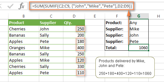
As you see, an array criteria makes the formula much more compact compared to SUMIF + SUMIF, and lets you add as many values as you like in the array.
This approach works with numbers as well as with text values. For instance, if instead of the suppliers' names in column C, you had supplier IDs like 1, 2, 3 etc., then your SUMIF formula would look similar to this:
=SUM(SUMIF(C2:C9, {1,2,3} , D2:D9))
Unlike text values, numbers needn't be enclosed in double quotes in array arguments.
Example 3. SUMPRODUCT & SUMIF
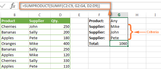
In case, your preferred way is to list the criteria in some cells rather that specify them directly in the formula, you can use SUMIF in conjunction with the SUMPRODUCT function that multiplies components in the given arrays, and returns the sum of those products.
=SUMPRODUCT(SUMIF(C2:C9, G2:G4, D2:D9))
Where G2:G4 are the cells containing your criteria, the suppliers' names in our case, as illustrated in the screenshot below.
But of course, nothing prevents you from listing the values in an array criteria of your SUMIF function if you want to:
=SUMPRODUCT(SUMIF(C2:C9, {"Mike","John","Pete"}, D2:D9))
The result returned by both formulas will be identical to what you see in the screenshot:
Excel SUMIFS with multiple OR criteria
If you want to conditionally sum values in Excel not simply with multiple OR conditions, but with several sets of conditions, you will have to use SUMIFS instead of SUMIF. The formulas will be very similar to what we've just discussed.
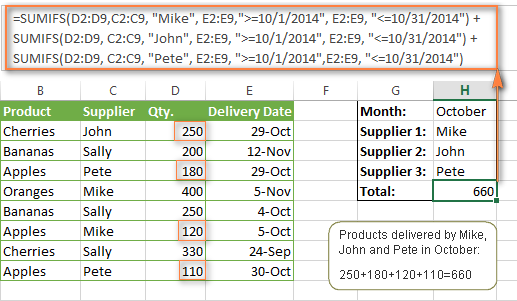
As usual, an example might help to illustrate the point better. In our table of fruit suppliers, let's add the Delivery Date (column E) and find the total quantity delivered by Mike, John and Pete in October.
Example 1. SUMIFS + SUMIFS
The formula produced by this approach includes a lot of repetition and looks cumbersome, but it is easy to understand and, most importantly, it works : )
=SUMIFS(D2:D9,C2:C9, "Mike", E2:E9,">=10/1/2014", E2:E9, "<=10/31/2014") +

SUMIFS(D2:D9, C2:C9, "John", E2:E9, ">=10/1/2014", E2:E9, "<=10/31/2014") +

SUMIFS(D2:D9, C2:C9, "Pete", E2:E9, ">=10/1/2014" ,E2:E9, "<=10/31/2014")
As you see, you write a separate SUMIFS function for each of the suppliers and include two conditions - equal to or greater than Oct-1 (">=10/1/2014",) and less than or equal to Oct 31 ("<=10/31/2014"), and then you sum the results.
Example 2. SUM & SUMIFS with an array argument
I've tried to explain the essence of this approach in the SUMIF example, so now we can simply copy that formula, change the order of arguments (as you remember it is different in SUMIF and SUMIFS) and add additional criteria. The resulting formula is more compact than SUMIFS + SUMIFS:
=SUM(SUMIFS(D2:D9,C2:C9, {"Mike", "John", "Pete"}, E2:E9,">=10/1/2014", E2:E9, "<=10/31/2014"))
The result returned by this formula is exactly the same as you see in the screenshot above.
Example 3. SUMPRODUCT & SUMIFS
As you remember, the SUMPRODUCT approach differs from the previous two in the way that you enter each of your criteria in a separate cell rather that specify them directly in the formula. In case of several criteria sets, the SUMPRODUCT function won't suffice and you will have to employ ISNUMBER and MATCH as well.
So, assuming that the Supplies Names are in cells H1:H3, Start Date is in cell H4 and End Date in cell H5, our SUMPRODUCT formula takes the following shape:
=SUMPRODUCT(--(E2:E9>=H4), --(E2:E9<=H5), --(ISNUMBER(MATCH(C2:C9, H1:H3,0))), D2:D9)
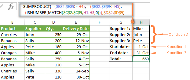
Many people wonder why use double dash (--) in SUMPRODUCT formulas. The point is that Excel SUMPRODUCT ignores all but numeric values, while the comparison operators in our formula return Boolean values (TRUE / FALSE), which are non-numeric. To convert these Boolean values to 1's and 0's, you use the double minus sign, which is technically called the double unary operator. The first unary coerces TRUE/FALSE to -1/0, respectively. The second unary negates the values, i.e. reverses the sign, turning them into +1 and 0, which the SUMPRODUCT function can understand.
I hope the above explanation makes sense. And even if it doesn't, just remember this rule of thumb - use the double unary operator (--) when you are using comparison operators in your SUMPRODUCT formulas.
Using Excel SUM in array formulas
As you remember, Microsoft implemented the SUMIFS function in Excel 2007. If someone still uses Excel 2003, 2000 or earlier, you will have to use a SUM array formula to add values with multiple AND criteria. Naturally, this approach works in modern versions of Excel 2013 - 2007 too, and can be deemed an old-fashioned counterpart of the SUMIFS function.
In the SUMIF formulas discussed above, you have already used array arguments, but an array formula is something different.
Example 1. Sum with multiple AND criteria in Excel 2003 and earlier
Let's get back to the very first example where we found out a sum of amounts relating to a given fruit and supplier:

As you already know, this task is easily accomplished using an ordinary SUMIFS formula:
=SUMIFS(C2:C9, A2:A9, "apples", B2:B9, "Pete")
And now, let's see how the same task can be fulfilled in early "SUMIFS-free" versions of Excel. First off, you write down all the conditions that should be met in the form of range="condition". In this example, we have two range/condition pairs:
Condition 1: A2:A9="apples"
Condition 2: B2:B9="Pete"
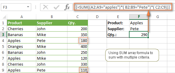
Then, you write a SUM formulas that "multiplies" all of your range/condition pairs, each enclosed in brackets. The last multiplier is the sum range, C2:C9 in our case:
=SUM((A2:A9="apples") * ( B2:B9="Pete") * ( C2:C9))
As illustrated in the screenshot below, the formula perfectly works in the latest Excel 2013 version.
Note. When entering any array formula, you must press Ctrl + Shift + Enter. Once you do this, your formula gets enclosed in {curly braces}, which is a visual indication that an array formula is entered correctly. If you try typing the braces manually, your formula will be converted to a text string, and it won't work.
Example 2. SUM array formulas in modern Excel versions
Even in modern versions of Excel, the power of the SUM function should not be underestimated. The SUM array formula is not simply gymnastics of the mind, but has a practical value, as demonstrated in the following example.
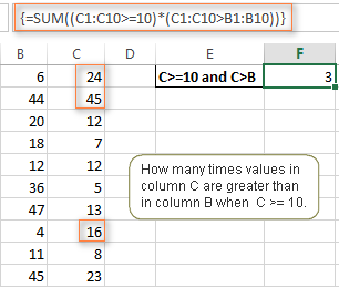
Suppose, you have two columns, B and C, and you need to count how many times column C is greater than column B, when a value in column C is greater or equal to 10. An immediate solution that comes to mind is using the SUM array formula:
=SUM((C1:C10>=10) * (C1:C10>B1:B10))
Don't see any practical application to the above formula? Think about it in another way : )
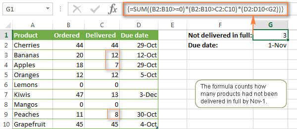
Suppose, you have the orders list like shown in the screenshot below and you want to know how many products have not been delivered in full by a given date. Translated into Excel's language, we have the following conditions:
Condition 1: A value in column B (Ordered items) is greater than 0
Condition 2: A value in column C (Delivered) in less than in column B
Condition 3: A date in column D (Due date) is less than 11/1/2014.
Putting the three range/condition pairs together, you get the following formula:
=SUM((B2:B10>=0)*(B2:B10>C2:C10)*(D2:D10<G2))
Well, the formula examples discussed in this tutorial have only scratched the surface of what Excel SUMIFS and SUMIF functions can really do. But hopefully, they have helped pointing you in the right direction and now you can sum values in your Excel workbooks no matter how many intricate conditions you have to consider.
 by
by
666 comments
I am trying to take overtime and regular hours out of one column and put into two columns.
i have all hours column that adds all the days total hours i would like to have my regular hour column take out everything up to 40 hours and then the OT column take everything over 40 hours. is that possible.
I'm interested in the same thing. Did you ever get a response?
Assuming the hours are in column A, you can use the following formulas to extract:
- Regular hours: =IF(A2<=40, A2, "")
- Overtime: =IF(A2>40, A2, "")
The screenshot below shows the result:
If you are looking for something different, please clarify.
Hi,
Resource Usage
Bob 50%
Mike 25%
Bob 75%
I would like to turn all Usage values for Bob RED when the sum exceed 100%. I know it is a SUMIF condition, but the syntax is alluding me. Any help would be appreciated.
Hello everyone,
I´m not sure which function to use to sum the products below in a different table.I tried to use the "sumif" function without sucess.
Products amounts Aples ?????
Aples 1500.00 Oranges ?????
oranges 400.00 Potatoes ?????
potatoes 590.00 Mango ?????
mango 522.00
oranges 789.00
Bananas 632.00
Aples 878.00
potatoes 965.00
Can anyone help me?
Hi Carlos,
The SUMIF function is the right choice. Supposing that column A is the list of products, B is Amounts and C is the product names in the second table (beginning in C2), you can use the following formula:
=SUMIF($A$2:$A$10, C2, $B$2:$B$10)
Hi Svetlana,
Im trying to apply same criteria for different columns (non adjacent), they are working well individually. Error occurs when I tried to add them together with the following formula.
=
SUMIFS(E18:E10000, G18:G10000, "John", I18:I10000, "01/07/2014”) +
SUMIFS(E18:E10000, K18:K10000, "John", M18:M10000, "01/07/2014”) +
SUMIFS(E18:E10000, O18:P10000, "John", Q18:Q10000, "01/07/2014”) +
SUMIFS(E18:E10000, S18:G10000, "John", U18:U10000, "01/07/2014")
Is there another way to add them without having to calculate individually (in different cells) and add. ?
- Ben
There was a typo in my earlier formula.
=
SUMIFS(E18:E10000, G18:G10000, "John", I18:I10000, "01/07/2014”) +
SUMIFS(E18:E10000, K18:K10000, "John", M18:M10000, "01/07/2014”) +
SUMIFS(E18:E10000, O18:O10000, "John", Q18:Q10000, "01/07/2014”) +
SUMIFS(E18:E10000, S18:S10000, "John", U18:U10000, "01/07/2014")
Hi can someone pls help me to count different criterias but in the same cell example if the followiing (math,bio,eng) (geo,math,) (bio,math,eng) in this case the bracket represent one cell but all those cells are in one column. My be 123 cells each having information of different subjects and now i want to count how many times each subject appears in that column. Remember the subjects are divided by commars in each cell. Pls i need to use this formular now friday if anyone can pls
I have given data in columns A and B
Column A column B
05/04/15 1
08/04/15 6
07/04/15 0
19/04/15 2
Actually I need to calculate the number of days from todays's date I mean count down.
but it must true 2 conditions for count down eg. whole range of column eg A2:A100 must be greater than todays date and whole range of column B eg. b2:b100 must be 1 then substract today's date with column A
Anyone can help, so I have on same sheet 12 different data filled tables for 12 months, on 13th table I would like to see cumulative sum of desired data. I woould like to choose to sum between february and june for example. Table is generated like 5X4 for every month where you can input data how many fruits (apples, bannanas, pears...) I have in different storages (1,2,3...) and would like to know how many fruits I have had between february and june. Hope someone understands and can help. Tnx
Excellent examples and explanations - congratulations on your expertise
This was a very useful article and was just what I was after - thank you!
Quick question, how can I use wildcards for the "Excel SUMIFS with multiple OR criteria" section please?
For example, if column C (Supplier) had a surname as well in the same cell, yet we still wanted to continue searching for just for forename, how would we do this using the formula from "Example 3. SUMPRODUCT & SUMIFS". I tried the following but it didn't work:
=SUMPRODUCT(--(E2:E9>=H4), --(E2:E9<=H5), --(ISNUMBER(MATCH(C2:C9, "*"&H1:H3&"*",0))), D2:D9)
Thanks.
Hello Svetlana,
Your explanation vis a vis the use of the Sumifs function was clear, straightforward, and immeasurably useful. I've been attempting to devise a method by which to accomplish the task that the Sumifs function can fulfill for the better part of three days (an attempt which led off in some pretty instructive, but ultimately futile directions). You have my sincere thanks for putting together a tutorial that I've little doubt required a fair degree of time and effort (not to mention the time that went into becoming an expert in the material in the first place). I can move forward with my project thanks to your work. Once more, thank you.
I WANT TO A FORMULA THAT HELP ME FOR CREATING BANK STATEMENT IN EXCEL SHEET .
FOR EXAMPLE:-THAT FORMULA ADD CREDIT SIDE WITH BANK BALANCE AND SUBTRACT DEBIT SIDE WITH AVAILABLE BANK BALANCE AUTOMATICALLY.
I need to count text within multiple tables from the start of the year to TODAY. The tables being each month and the text being vacation days "V" in each cell. I'm having trouble defining the date in the range. The each cell in the top row has the following format:
=TEXT(WEEKDAY(DATE(CalendarYear,3,9),1),"aaa")
The first column is the employees name.
I found the SUMIF function for adding using the date criteria, and the COUNTIF function the count the text "V". I'm having trouble combining the two.
Thanks
Thank you so much for your wonderful, clear easy to follow tutorials :) I have learnt so much and am amazed at how quickly I have done that!!!
How to automate the below process?
Parameter 2
Week 1 Week 2 Week 3 Week 4 Week 5 Week 6 Week 7 Week 8 Week 9 Week 10
Sales 10 10 10 10 5 5 5 5 5 5
WOC 20 20 20 15 10 10 10 10 10 5
if I vary parameter=4, woc on Wk1=40(consider first weeks sum)
Wk2=35
Please help
I want a formula that will add up all the numbers but only if it has a B. What would be the best formula for that? I would like to and the number and letter all in once cell so it would look something like this.
7B
6B
1R
I have created the following array formula which works fine to summ based on the multiple GL accounts. Now i want to add another criteria in to the formula to only sum based on months. My data is in a list from and it is for 12 months. The idea is that formula will look at the header for name month and than only sum relevant dollars in to the column.
Col H = dollars, Col D = GL account, Col A = Month
=SUM(SUMIFS('GL Data'!$H:$H,'GL Data'!$D:$D,{"400000","400550","430260","400500","403000","403010","403505","404500"}))
Please help. Rashid
I'm looking for a formula that tell me how many time it replaced the same part in different cars. see chart
Car # Replaced Parts
Car 1 Battery
Car 5 Gas Tank
Car 3 Windsheild
Car 4 Battery
Car 5 Gas Tank
Car 2 Battery
Car 4 Lock
Car 1 Filter
Car 1 Battery
Car 5 Windsheild
Car 3 Gas Tank
I replace the Gas Tank 3 time in different (2) cars. But I want to know how many times I replace the Gas Tank in different cars.
Thanks in advance.
CAN YOU HELP WITH A FORMULA TO DETERMINE THE NUMBER OF TIMES "NO SHOW OR CX" APPEARS IN RELATION TO A CELL? FOR EXAMPLE TEXT IN CELLS L40:L150 SPLIT
CELLS N40:N150 WOULD HAVE EITHER CX OR NOW SHOW LISTED CAN I GET A FORMULA INDICATING A TOTAL OF NO SHOW AND CX WITHOUT ADDING ANOTHER COLUMN?
THIS IS WHAT i HAVE TRIED BUT CANNOT GET IT TO WORK:
=COUNTIFS(L40:L150,"SPLIT",N40:N150,"NO SHOW",N40:N150,"CX")
if there is a error cell in the sum range then how we will use this formula
M5 is Starting Date and I5 is Ending date
=SUMIFS(SAmount,SItmName,H8,SaleDate,">=M5",SaleDate,"<=I5")
I am writing sumifs formula in that way but it did not calculate, Please one who help me regarding to this
Thanks
Good post, thanks. I have a followup question. I am currently using this SUMIF($D$3:$D$22,"=1",$B$3:$B$22). Now instead of =1, if I want to provide a cell location it doesnt work. How do I do this? For example, SUMIF($D$3:$D$22,"=K43",$B$3:$B$22)
Any idea on this? When I try this it calculates incorrectly. Do I need to use quotes differently?
Hello Arun R,
I had the same problem and solved it as per the below change.
SUMIF($D$3:$D$22,"="&K43,$B$3:$B$22)
Hope it works for you too!
i think i'm over thinking it but I can not get the either or value to function
column g has Yes or no in column h i want it to look at column g and if it is yes populate $250 if it is no populate $150. =IF(G41="NO",150,)*OR(G41="yes",250)
the yes is giving a $0.0 result.
What am I doing wrong?
Help!
Column F = Account Coding Letters ( I will input data into this resembling an account code e.g 001)
Column G = Production coding Letters (I will input data into this resembling initials for someones name e.g PH)
Column H = Net Price of what is spent (e.g £25
Column K = NEEDS TO BE ABLE TO INPUT ANY CODING LETTER FROM EITHER COLUMN F OR G
Column L = Needs to take the sum of the net price that is related to the coding letter that is inputed from column K.
For example say if Polly Holloway bought fuel and I have an account code for fuel that is 001 and an initial code for Lauren which is LH)
I need to be able to input into column L either of the codes 001 or PH (They will never be input together in the same cell) All I need to know how many times Polly bought fuel on our company and how many times fuel was bought altogether.
So in a sense column K needs to be have a range of columns F & G
At the moment the formula I have in column L is only applicable to Column G.
Please see below:
=SUMIF(G$9:G$44,K23,H$9:H$44)
What is the formula that I can put into Column L so it applies to both Column G & Column F?
Please help!
I am using a formula in Excel spreadsheets that works great but it doesn't work in Excel 2003. Can you tell me what formula I need to use in 2003 - 2007 to get the same result as excel 2010
=SUMIFS(D2:D80,$B$2:$B$80,"Overtime Paid",D2:D80,">0:00")
I am using a formula in Excel spreadsheets that works great but it doesn't work in Excel 2003. Can you tell me what formula I need to use in 2003 - 2007 to get the same result as excel 2010
=SUMIFS(D2:D80,$B$2:$B$80,"Overtime Paid",D2:D80,">0:00")
What if I don't want to sum? What if I am looking at listing the commissions that a salesperson received and for what company they sold to. Let's say that the salesperson has a code - 1, 2, 3 and so on, in column A. The customer name is in column B. I want the formula to read column A to the bottom and return the name of every customer they sold to in another tab in column H. The answer would look like this;
Salesperson Customer
7 Apple, McDonalds, Chevron
Can you tell me what the formula would be for that?
Thanks!
Valerie
Hi,
I am having an issue but not 100% if this solves it or not. It involves trying to have different sums performed based on multiple selection criteria.
The idea is to have 2 criteria which can be selected by dropdown lists. The user simply picks the 2 criteria and then places an "X" in the rows he requires. The pricing calculator then works out a cost.
For example if a certain service (Service A, Service B, Service C) is selected from a dropdown list, and a currency is selected from the second drop down list then perform a certain calculation based on thatcriteria.
In this example, if Service A is selected with currency = "GBP" then it would perform a sumif from the GBP price column for that service. If Service A is selected with currency = USD, it will perform a sumif from the USD price column for that service.
I have it working for when only one criteria is applied but cannot seem to get it for both. In the below formula, column B is where the user puts "x" in and then column K has the GBP cost. The formula needs to use a different column for the USD cost (column L).
=IF(G6="Service A",SUMIF(B21:B117,"x",K21:K117), "")
the above formula should read something like IF G6 =Service A AND G7 = "GBP" then do the sum using column K. IF G6 = Service A AND G7 = "USD" then do the sum but using column L.
If anyone knows how to do this, any help would be appreciated.
Thanks
Stephen
I am trying to calculate more than one quantity but cant find the formula to use. Example in column d I have quantity in column e I have Retail price in column e I would like for the total of all the quanitiy at a total. Please help
Very Helpful Svetlana!
hi Svetlana, this was a great post!
i'm hoping you can help me out on a quick question. you used an array argument in your formula in Example 2 of 'Excel SUMIFS with multiple OR criteria'
my question is, how can i reference an array argument from a cell, instead of typing it in a formula:
i want to reference the array argument {"Mike", "John", "Pete"} from just one cell instead of in a formula as you have in the following:
SUM(SUMIFS(D2:D9,C2:C9, {"Mike", "John", "Pete"}, E2:E9,">=10/1/2014", E2:E9, "<=10/31/2014"))
thanks for any help on this!
This is what I used and it worked, but I'm kind of skeptical.
=SUMPRODUCT(C3:C19,$D3:$D19)
I have column B and C of % weight that correspond with $figure in column D. Column B belongs to partner Arthur and Column B belongs to partner Roxy. Column D has total annual expenses for each category e.g. Travel, Computer Purchase...
How would I construct a formula to look into column B identify the % weight, multiply it to $ figure in Column D and sums up the result. Keep in mind that each % weight in the cell can be different so the formula has to identify the weight and than get the corresponding dollar figure for each cell and sum those up together.
Hello Vince,
I am sorry, it is quite difficult to understand the task without seeing your data. If you can send a small sample workbook to support@ablebits.com, we’ll be able to assist you better.
Any Body can help me to calcuate this
in A column have product name
in B have its price
in C column have mention its quantity
that database is to 13 rows
i want grand total of B multipal with C of each row.
Thank You
Hello Abdul,
=SUMPRODUCT(B2:B13,C2:C13)
Hello Abdul,
Please use the SUMPRODUCT function:
=sumproduct(B2:B13,C2:C13)
You can find more information about SUMPRODUCT here:
https://support.office.microsoft.com/en-us/article/SUMPRODUCT-function-57a7bfa7-f74d-4ead-8c93-57f759c8f616
I am new to SUMIFS functions but seem to be following the formula but get incorrect result.
Using 2 worksheets in the spreadsheet.
First Worksheet - multiple entries for each contract
Column A contract number
Column B Date
Column C Costs (Amount)
second worksheet - one entry for each contract
Column A contract number
Column B Date
So in the 2nd worksheet I want to sum all costs (on 1st worksheet) for each contract that occured after a certain date.
So I have tried the following forumla
SUMIFS(worksheet1$C$1:$C$2000),worksheet1$A$1:$A$20000,worksheet2"$A2",worksheet1$B$1:$B$20000,">=worksheet 1$B2")
When I leave the date criteria off I get the correct figure for the complete total but when I try to add the date criteria I get a value of 0.
Hello Rachel,
Please use this formula:
=SUMIFS(worksheet1!$C$1:$C$2000,worksheet1!$A$1:$A$20000,worksheet2!$A2,worksheet1!$B$1:$B$20000,">="&worksheet1!$B2)
Most likely the issue is due to this part: ">="&worksheet1!$B2
I was having the same problem as Rachel. Alexander's solution worked for me. Stills seems like unnecessarily complicated syntax, but it works.
Hi Svetlana
Column A: Project ref
Column B: Total hours on Project in one day
Column C: Total hours on one project overall
Rows = Days of the week
Column A consists of multiple reference numbers which repeat if a project is worked on for more than one day, but not necessarily on consecutive days. I want to be able to cumulatively add the total hours worked on a project over multiple days using a sumif calculation. For example i would like the total number of hours worked on project ref 222 over several non consecutive days in one month. The project ref range is large and therefore i do not want to specify "222" in the criteria but all instances where a reference number is repeated in the ref column.
Can you please help.
Thanks
Dan
can i have some examples of SUMIF with IF ??
also COUNTIFS with IF ??
Could you please clarify what examples you need? We have several articles about these functions:
https://www.ablebits.com/office-addins-blog/if-function-excel/
https://www.ablebits.com/office-addins-blog/excel-and-or-xor-not-functions/
https://www.ablebits.com/office-addins-blog/excel-not-equal-to-greater-than-less-than/
https://www.ablebits.com/office-addins-blog/excel-if-function-multiple-conditions/
I sold 3 plums, 6 apples and 4 pears on the 6th Jan. How do I total the amount of fruit sold on any given day. So in my example, "How many items of fruit did I sell on the 6th Jan?" The result would be 13, i.e. I sold 13 items of fruit on the 6th Jan.
I wish I could send you the actual excel document but looks tricky to paste it here
Variable Formulae Value
HYTRW 5453
JDGFSW 4356
YREDV 5858
ACFV REEEE+K533EG-JLIULM 14633
MHKYU 6878
NTRGV 5433
SVEDH -HYTRW+NTRGV-+BBCVB-JDGFSW -8031
BDHRYH 3213
K533EG 9078
JLIULM 3335
SGEEG GTGS+BDHRYH 7680
WGTHR 7886
BBCVB 3655
VB CVNN 5444
GTGS 4467
REEEE 8890
I have a problem with excels sumifs function. am trying to add information in Column B that is appearing also in Column A and those in column A have values in Column C.
Suppose there are 1000 entries in column A and you want to add some of them based on a function containing information in column B and find the total. How can I proceed? Example; find sum of AAAA+bbbG-JHFG+THRYR where these are infor in column A but spread across that searching for them can be cumbersome and the total should be based on their individual values in col C and results appearing in column D. Can you help me with this please?
Column A B C D
dsgsg
grhhht
AAAA
FGGGET
Dear Sir,
I am looking for to choose a particular rate if for many specific ranges. For example:
0 - 350 Kg = rate 2.5
350 - 500 Kg = rate 1.9
500 - 800 Kg = rate 1.8
800 - Above rate 1.68
So how do i apply this
IF(A10>800,1.68,IF(A10>500,1.8,IF(A10>350,1.9,2.5)))
Region Amount
Zone 1 1
Zone 1 2
Zone 1 3
Zone 1 4
Zone 1 5
Zone 1 6
Zone 1 7
Zone 1 8
Zone 1 9
Zone 1 10
Zone 2 1
Zone 2 2
Zone 2 3
Zone 2 4
Zone 2 5
Zone 2 6
Zone 2 7
Zone 2 8
Zone 2 9
Zone 2 10
Zone 2 11
Zone 2 12
Zone 2 13
Zone 2 14
Zone 2 15
Franchisee 1
Franchisee 2
Franchisee 3
Franchisee 4
Franchisee 5
Franchisee 6
Franchisee 7
Franchisee 8
Franchisee 9
Franchisee 10
Franchisee 11
Franchisee 12
Franchisee 13
Franchisee 14
Franchisee 15
Franchisee 16
Franchisee 17
Franchisee 18
Franchisee 19
Franchisee 20
I want Top 5 Sum with Region (Zone 1 - 40, Zone 2 - 65 and Franchisee - 90), Kindly provide the formula fo this
Thank You!!!...
I need to do something similar to the formula you provided, but instead of:
=SUM(SUMIF(C2:C9, {1,2,3} , D2:D9))
I want to do:
=SUM(SUMIF(C2:C9, {A9,A10,A14} , D2:D9))
But it gives me an error. Could you please advise if there is a way to use a cell reference instead of a string or constant?
Thank you!!!
The cell selections will have to be continuous and then you can use array formula for this:
=SUM(SUMIF(C2:C9, A9:A14 , D2:D9))
type the formula and hit ctrl+enter
curly braces will appear around your formula:
{=SUM(SUMIF(C2:C9, A9:A14 , D2:D9))}
I've tried to use this in two different ways but both methods fail to provide the correct answer:
Method 1)
Formula:
=SUM(SUMIFS('Personal History Data Dump'!$J$2:$J$16000,'Personal History Data Dump'!$F$2:$F$16000,'Daily Roster'!$A4,'Personal History Data Dump'!$C$2:$C$16000,Categories!B$4:B$17))
Problem: Only Sums based on the first criteria in Categories!B$4:B$17. Adding "{}" brackets around "Categories!B$4:B$17" only results in an error asking me if I'm not trying to enter a formula into the cell.
Method 2)
Formula:
=SUM(SUMIFS('Personal History Data Dump'!$J$2:$J$16000,'Personal History Data Dump'!$F$2:$F$16000,'Daily Roster'!$A4,'Personal History Data Dump'!$C$2:$C$16000,{Categories!B$4,Categories!B$5,Categories!B$6,Categories!B$7,Categories!B$8,Categories!B$9,Categories!B$10,Categories!B$11,Categories!B$12,Categories!B$13,Categories!B$14,Categories!B$15,Categories!B$16,Categories!B$17}))
Problem: Returns the same error mentioned above, asking me if I'm not trying to enter a formula into the cell. It specifically highlights the first "Categories" reference as an issue.
I've used this exact formula before with success, but instead of referencing cells I inserted specific values between the "{}" brackets. For example, the portion in the brackets looked like this: {">5000","<20000"}.
Is Excel just not recognizing the cell references as cell references? If so, is there any way to get around that?
I want indirect to reference a cell E3 containing {"Cherry","Tomatoes"}
that can be used in a sumproduct+sumif formula like the one below.
=sumproduct(sumif(c2:c10,D2:d10,indirect("E3")))
hi K, did you ever figure this out? i want to do the same.
Did you figure this out? That's exactly what I'm trying to do... I want to reference the array "text" in a separate cell from my formula to make it easier to update, or so I could choose to use a single value instead of an array. Is it possible?
hi, i also have the same issue, is there a solution where i can refer to the text in few cells or in a single cell seperated with ","
thanks
i want to make a surgical regt.& next sheet or same page report format to auto generate. Regt cell -Sex, next cell -Ulcer,next cell -debridement than nex cell -Rt.Hand/Rt.foot ctc .
in reporting format- to result if male(sex wise) /rt.hand (operated)/Lt.foot (operated)etc.
please help for it. to make in excel
.
thanks.
Any buddy has used "SUMIFS" command with "CONTAIN"
you can use the following to simulate contain:
"*"&"whatever you think it needs to contain"&"*"
Adding the "*"& or &"*" allow excel to look for any for any wildcards in front or after the string you want.
Ablebits is an website an excellent teacher ,for the beginners.
I have learn more than a lot.I want to subscribe to this website for receiving the daily updates to become awesome in microsoft office Professional product.
Hello Svetlana,
Please help me. How to use Sumif() function, when RANGE (f.e. 4042-5201) and CRITERIA (f.e. 4042) does not equal to each other? In the CRITERIA I have 4042 and need to SUM figures in the RANGE with value 4042-5201.
Thanks in Advance.
Beso
For your Numbers:
=SUMIFS(sum_range;criteria_range1;">=4042";criteria_range1;"="&G4;$B$4:B32;"<"&G5)
For your Numbers:
=SUMIFS(sum_range;criteria_range1;">=4042";criteria_range1;"="&G4;criteria_range1;"<"&G5)
Hope this is helpefull to someone ☺
Last try If my entire post is not showing now, i will give up
For your Numbers:
=SUMIFS(sum_range;criteria_range1;">=4042";criteria_range1;"="&G4;criteria_range1;"<"&G5)
I Hope this is helpefull to someone ☺
Hi Svetlana,
I made a mistake in asking my question! The SUMIFS formula you gave is for cherries AND john. If I want cherries OR john (OR function between column A and B). I am working on a spreadsheet that has a SUM(SUMIFS...) I have multiple columns that have overlapping data, so instead of using AND logic I need to use OR logic between the columns themselves.
Thanks
Got it! Then you can add up several SUMIF fucntions, like this:
=SUMIF(A:A, "cherries", C:C) + SUMIF(B:B, "john", C:C)
that is not correct
=SUMIF(A:A,"cherries",C:C)+SUMIFS(C:C,B:B,"john",A:A,"cherries")
or you could do:
=SUMIF(A:A, "cherries", C:C) + SUMIF(B:B, "john", C:C) - SUMIFS(C:C,B:B,"john",A:A,"cherries")
Algebra has several solutions here that are all equivalent. The solution above mine is actually slightly shorter in terms of formula.
IF you want to total how many cherries were supplied by John (OR function between columns A & B instead of OR function between values in a given column) how could you organize the forumula?
Hello Becca,
In Excel 2007-2013, you can use the following SUMIFS formula (column C is Qty., column A - product and column B - supplier):
=SUMIFS(C:C, A:A, "cherries", B:B, "john")
In earlier Excel versions, you will have to use an array SUM instead (remember to press Ctrl +Shift + Alt):
=SUM((A2:A9="cherries") * ( B2:B9="john") * ( C2:C9))
I'm trying this formula but its not working on my sheet
=SUMIFS(I10:I88,G10:G88,"AGO - PETROL",H10:H88,"874")
My table has all the columns but when pressing enter key to get the
result comes a #value . Can anyone help me knowing the problem?
Instead of SUMIFS you should use SUMIF in this case