The tutorial explains what an Excel name is and shows how to define a name for a cell, range, constant or formula. You will also learn how to edit, filter and delete defined names in Excel.
Names in Excel are a paradoxical thing: being one of the most useful features, they are often considered pointless or nerdy. The reason is that very few users understand the essence of Excel names. This tutorial will not only teach you how to create a named range in Excel, but will also show how to leverage this feature to make your formulas much easier to write, read, and re-use.
What does name mean in Excel?
In everyday life names are widely used to refer to people, objects and geographical locations. For example, instead of saying "the city lying at latitude 40.7128° N and longitude 74.0059° W, you simply say "New York City".
Similarly, in Microsoft Excel, you can give a human-readable name to a single cell or a range of cells, and refer to those cells by name rather than by reference.
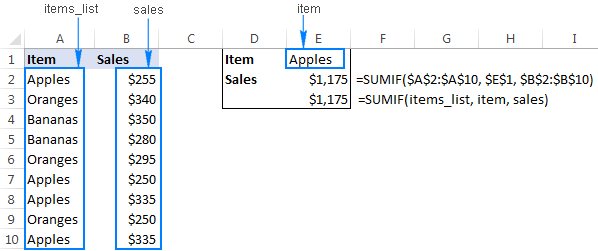
For instance, to find the total of sales (B2:B10) for a specific item (E1), you can use the following formula:
=SUMIF($A$2:$A$10, $E$1, $B$2:$B$10)
Or, you can give meaningful names to the ranges and individual cells and supply those names to the formula:
=SUMIF(items_list, item, sales)
Looking at the screenshot below, which of the two formulas are easier for you to understand?
Excel name types
In Microsoft Excel, you can create and use two types of names:
Defined name - a name that refers to a single cell, range of cells, constant value, or formula. For example, when you define a name for a range of cells, it's called a named range, or defined range. These names are subject of today's tutorial.
Table name - a name of an Excel table that is created automatically when you insert a table in a worksheet (Ctrl + T). For more information about Excel tables, please see How to make and use a table in Excel.
How to create an Excel named range
Overall, there are 3 ways to define a name in Excel: Name Box, Define Name button, and Excel Name Manager.
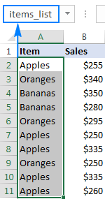
Type a name in the Name Box
The Name Box in Excel is fastest way to create a named range:
- Select a cell or a range of cells that you want to name.
- Type a name into the Name Box.
- Press the Enter key.
Voila, a new Excel named range is created!
Create a name by using the Define Name option
Another way to make a named range in Excel is this:
- Select the cell(s).
- On the Formulas tab, in the Define Names group, click the Define Name button.
- In the New Name dialog box, specify three things:
- In the Name box, type the range name.
- In the Scope dropdown, set the name scope (Workbook by default).
- In the Refers to box, check the reference and correct it if needed.
- Click OK to save the changes and close the dialog box.
Note. By default, Excel creates a name with absolute references. If you'd rather have a relative named range, remove the $ sign from the reference (before you do this, make sure you fully understand how relative names behave in worksheets).
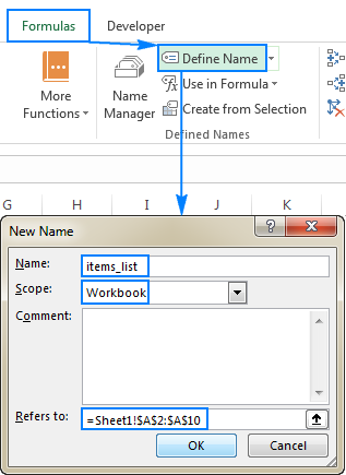
Compared to the previous method, using Define Name in Excel takes a few extra clicks, but it also provides a couple more options such as setting the name's scope and adding a comment that explains something about the name. Additionally, Excel's Define Name feature allows you to create a name for a constant or formula.
Make a named range by using Excel Name Manager
Usually, the Name Manager in Excel is used to work with existing names. However, it can help you build a new name too. Here's how:
- Go to the Formulas tab > Defined Names group, click Name Manager. Or, just press Ctrl + F3 (my preferred way).
- In the top left hand corner of the Name Manager dialog window, click the New… button:
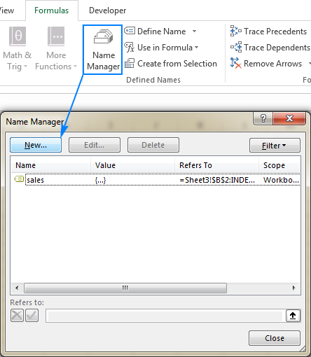
- This will open the New Name dialog box where you configure a name as demonstrated in the previous section.
Tip. To quickly test the newly created name, select it in the Name Box dropdown list. As soon as you release the mouse, the range on the worksheet will be selected.
How to create an Excel name for a constant
In addition to named ranges, Microsoft Excel allows you to define a name without cell reference that will work as a named constant. To create such a name, use either the Excel Define Name feature or Name Manager as explained above.
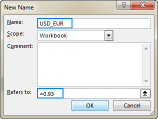
For instance, you can make a name like USD_EUR (USD - EUR conversion rate) and assign a fixed value to it. For this, type the value preceded by an equal sign (=) in the Refers to field, e.g. =0.93:
And now, you can use this name anywhere in your formulas to convert USD to EUR:
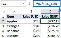
As soon as the exchange rate changes, you update the value only in one central location, and all of your formulas will get recalculated in a single step!
How to define a name for a formula
In a similar manner, you can give a name to an Excel formula, for example, the one that returns the count of non-empty cells in column A, excluding the header row (-1):
=COUNTA(Sheet5!$A:$A)-1
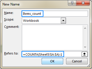
Note. If your formula refers to any cells on the current sheet, you do not need to include the sheet name in the references, Excel will do it for you automatically. If you are referencing a cell or range on another worksheet, add the sheet's name followed by the exclamation point before the cell/range reference (like in the formula example above).
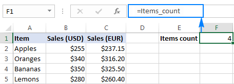
Now, whenever you want to know how many items there are in column A on Sheet5, not including the column header, just type the equality sign followed by the name of your formula in any cell, like this: =Items_count
How to name columns in Excel (names from selection)
If your data is arranged in a tabular form, you can quickly create names for each column and/or row based on their labels:
- Select the entire table including the column and row headers.
- Go to the Formulas tab > Define Names group, and click the Create from Selection button. Or, press the keyboard shortcut Ctrl + Shift + F3.
- Either way, the Create Names from Selection dialogue box will open. You select the column or row with headers, or both, and click OK.
In this example, we have headers in the top row and left column, so we select these two options:
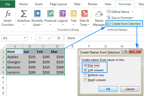
As the result, Excel will create 7 named ranges, picking up names from the headers automatically:
- Apples, Bananas, Lemons and Oranges for rows, and
- Jan, Feb and Mar for columns.

Note. If there are any spaces between words in the header labels, the spaces will be replaced with underscores (_).
Excel dynamic named range
In all previous examples, we have been dealing with static named ranges that always refer to the same cells, meaning you would have to update the range reference manually whenever you want to add new data to the named range.
If you are working with expandable data sets, it stands to reason to create a dynamic named range that accommodates newly added data automatically.
The detailed guidance on how to create a dynamic named range in Excel can be found here:
Excel naming rules
When creating a name in Excel, there are a few rules to remember:
- An Excel name should be under 255 characters long.
- Excel names cannot contain spaces and most punctuation characters.
- A name must begin with a letter, underscore (_), or backslash (\). If a name begins with anything else, Excel will throw an error.
- Excel names are case-insensitive. For example, "Apples", "apples" and "APPLES" will be treated as the same name.
- You cannot name ranges like cell references. That is, you can't give the name "A1" or "AA1" to a range.
- You can use a single letter to name a range like "a", "b", "D", etc. except for the letters "r" "R", "c", and "C" (these characters are used as shortcuts for selecting a row or column for the currently selected cell when you type them in the NameBox).
Excel name scope
In terms of Excel names, scope is the location, or level, within which the name is recognized. It can be either:
- Specific worksheet - the local worksheet level
- Workbook - the global workbook level
Worksheet level names
A worksheet-level name is recognized within the worksheet where it is located. For example, if you create a named range and set its scope to Sheet1, it will be recognized only in Sheet1.
To be able to use a worksheet-level name in another worksheet, you must prefix the worksheet's name followed by the exclamation point (!), like this:
Sheet1!items_list
To reference a worksheet-level name in another workbook, you should also include the workbook name enclosed in square brackets:
[Sales.xlsx]Sheet1!items_list
If either the sheet name or workbook name contains spaces, they should be enclosed in single quotation marks:
'[Sales 2017.xlsx]Sheet1'!items_list
Workbook level names
A workbook-level name is recognized within the entire workbook, and you can refer to it simply by name from any sheet in the same workbook.
A use to a workbook-level name in another workbook, precede the name with the workbook name (including the extension) followed by the exclamation point:
Book1.xlsx!items_list
Scope precedence
A defined name must be unique within its scope. You can use the same name in different scopes, but this might create a name conflict. To prevent this from happening, by default, the worksheet level takes precedence over the workbook level.
If there are a few identically named ranges with different scopes, and you want to use the workbook level name, prefix the name with the workbook name as if you were referring to a name in another workbook, e.g.: Book1.xlsx!data. This way, the name conflict can be overridden for all worksheets except for the first sheet, which always uses the local worksheet level name.
Excel Name Manager - quick way to edit, delete and filter names
As its name suggests, the Excel Name Manager is specially designed to manage names: change, filter, or delete existing names as well as create new ones.
There are two ways to get to the Name Manager in Excel:
- On the Formulas tab, in the Define Names group, click the Name Manager
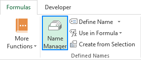
- Press the Ctrl + F3 shortcut.
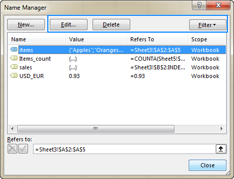
Either way, the Name Manager dialog window will open, letting you see all names in the current workbook at a glance. Now, you can select the name you want to work with, and click one of the 3 buttons at the top of the window to perform the corresponding action: edit, delete or filter.
How to edit named range in Excel
To change an existing Excel name, open the Name Manager, select the name, and click the Edit… button. This will open the Edit Name dialog box where you can change the name and reference. The scope of the name cannot be changed.
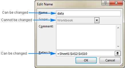
To edit a name reference, you do not need to open the Edit Name dialog box. Just select the name of interest in the Excel Name Manager, and type a new reference directly in the Refers to box, or click the button at the right and select the desired range on the sheet. After you click the Close button, Excel will ask if you want to save the changes, and you click Yes.
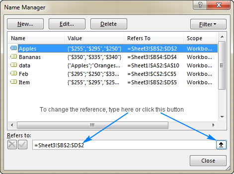
Tip. An attempt to navigate through a long reference or formula in the Refers to field with the arrow keys will most likely result in a very frustrating behavior. To move within this field without disrupting the reference, press the F2 key to switch from Enter to Edit mode.
How to filter names in Excel
If you have a lot of names in a certain workbook, click the Filter button at the top right corner of the Excel Name Manager window to view only the names relevant at a given time. The following filters are available:
- Names scoped to worksheet or workbook
- Names with or without errors
- Defined names or table names
How to delete named range in Excel
To delete a named range, select it in the Name Manager and click the Delete button at the top.
To delete several names, click the first name, then press the Ctrl key and hold it while clicking other names you want to remove. Then click the Delete button, and all selected names will be deleted in one go.
To delete all defined names in a workbook, select the first name in the list, press and hold the Shift key, and then click the last name. Release the Shift key and click Delete.
How to delete defined names with errors
If you have a number of invalid names with reference errors, click the Filter button > Names with Errors to filter them:
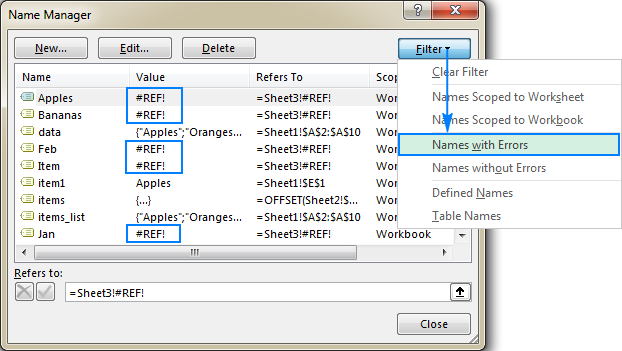
After that, select all filtered names as explained above (by using the Shift key), and click the Delete button.
Note. If any of your Excel names are used in formulas, be sure to update the formulas before deleting names, otherwise your formulas will return #NAME? errors.
Top 5 benefits of using names in Excel
So far in this tutorial, we have been focusing mostly on how-to things that cover different aspects of creating and using named ranges in Excel. But you may be curious to know what is so special about Excel names that makes them worth the effort? The top five advantages of using defined names in Excel follow below.
1. Excel names make formulas easier to make and read
You don't have to type complex references or go back and forth selecting ranges on the sheet. Just start typing the name you want to use in the formula, and Excel will show a list of matching names for you to choose from. Double click the desired name, and Excel will insert it in the formula straight away:

2. Excel names allow creating expandable formulas
By using dynamic named ranges, you can create a "dynamic" formula that automatically includes new data in calculations without you having to update every reference manually.
3. Excel names make formulas easier to re-use
Excel names make it a lot easier to copy a formula to another sheet or port a formula into a different workbook. All you have to do is create the same names in the destination workbook, copy/paste the formula as is, and you will get it working immediately.
Tip. To prevent Excel form creating new names on the fly, copy the formula as text in the formula bar instead of copying the formula cell.
4. Named ranges simplify navigation
To quickly get to a specific named range, just click on its name in the Name box. If a named range resides on another sheet, Excel will take you to that sheet automatically.
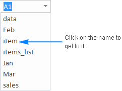
Note. Dynamic named ranges do not show up in the Name box in Excel. To see dynamic ranges, open the Excel Name Manager (Ctrl + F3) that shows full details about all names in the workbook, including their scope and references.
5. Named ranges allow creating dynamic drop-down lists
To build an expandable and updatable drop down list, make a dynamic named range first, and then create a data validation list based on that range. The detailed step-by-step instructions can be found here: How to create a dynamic dropdown in Excel.
Excel named range - tips and tricks
Now that you know the basics of creating and using names in Excel, let me share a few more tips that may prove helpful in your work.
How to get a list of all names in the workbook
To get a more tangible list of all names in a current workbook, do the following:
- Select the topmost cell of the range where you want the names to appear.
- Go to the Formulas tab > Define Names group, click Use in Formulas, and then click Paste Names… Or, simply press the F3 key.
- In the Paste Names dialog box, click Paste List.
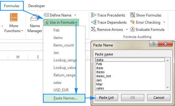
This will insert all Excel names along with their references in the current worksheet, beginning in the selected cell.
Absolute Excel names vs. relative Excel names
By default, Excel names behave like absolute references - locked to specific cells. However, it is possible to make a named range relative to the position of the active cell at the time the name is defined. Relative names behave like relative references - get changed when the formula is moved or copied to another cell.
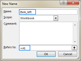
In fact, I cannot think of any reason why one would want to make a relative named range, except maybe when a range consists of a single cell. As an example, let's create a relative name that refers to a cell one column to the left of the current cell, in the same row:
- Select cell B1.
- Press Ctrl + F3 to open Excel Name Manager, and click the New…
- In the Name box, type the desired name, say, item_left.
- In the Refers to box, type
=A1. - Click OK.
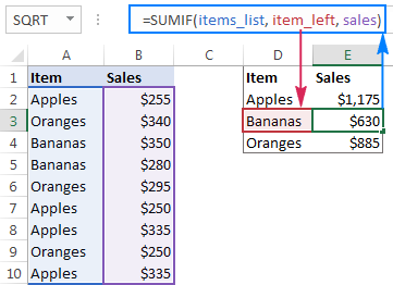
Now, let's see what happens when we use the item_left name in a formula, for example:
Where items_list refers to $A$2:$A$10 and sales refers to $B$2:$B$10 in the table below.
When you enter the formula in cell E2, and then copy it down the column, it will calculate the total sales for each product individually because item_left is a relative name and its reference adjusts based on the relative position of the column and row where the formula is copied:
How to apply Excel names to existing formulas
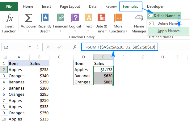
If you've defined the ranges that are already used in your formulas, Excel won't change the references to the appropriate names automatically. Though, instead of replacing references with names by hand, you can have Excel do the work for you. Here's how:
- Select one or more formula cells that you want to update.
- Go to the Formulas tab > Define Names group, and click Define Name > Apply Names…
- In the Apply Names dialog box, click on the names you want applied, and then click OK. If Excel is able to match any of the existing names with the references used in your formulas, the names will be selected for you automatically:
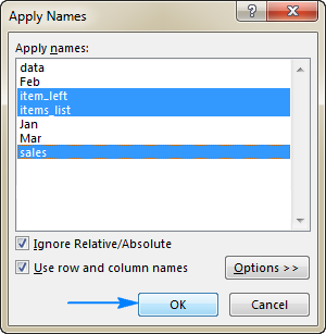
Additionally, two more options are available (selected by default):
- Ignore Relative/Absolute - keep this box checked if you want Excel to apply only the names with the same reference type: replace relative references with relative names and absolute references with absolute names.
- Use row and column names - if selected, Excel will rename all cell references that can be identified as the intersection of a named row and named column. For more choices, click the Options
Excel name shortcuts
As is often the case in Excel, the most popular features can be accessed in several ways: via the ribbon, right-click menu, and keyboard shortcuts. Excel named ranges are no exception. Here are three useful shortcuts to work with names in Excel:
- Ctrl + F3 to open the Excel Name Manager.
- Ctrl + Shift + F3 to create named ranges from selection.
- F3 to get a list of all Excel names in a workbook.
Excel name errors (#REF and #NAME)
By default, Microsoft Excel does its best to keep your defined names consistent and valid by adjusting range references automatically when you insert or delete cells within an existing named range. For example, if you have created a named range for cells A1:A10, and then you insert a new row anywhere between rows 1 and 10, the range reference will change to A1:A11. Similarly, if you delete any cells between A1 and A10, your named range will contract accordingly.
However, if you delete all cells that make up an Excel named range, the name becomes invalid and displays a #REF! error in the Name Manager. The same error will show up in a formula referencing that name:
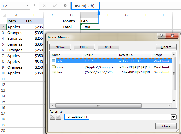
If a formula refers to a non-existing name (mistyped or deleted), the #NAME? error will show up. In either case, open the Excel Name Manager and check the validity of your defined names (the fastest way is to filter names with errors).
This is how you create and use names in Excel. I thank you for reading and hope to see you on our blog next week!
 by
by
107 comments
Sorry one more thing: I have been very careful not to use any volatile functions in these formulas.
I am a big fan of your blog and advice.
My question: I am trying to figure out the relative efficiencies of:
-Using a reasonably complex array formula [Complex Formula] many times throughout a worksheet, sometimes directly, sometimes as an intermediate calculation for some more complex formulas;
-Putting [Complex Formula] into a dynamic named range and using the named range throughout the worksheet;
-Storing [Complex Formula] in a particular location in the worksheet and referring to it when needed by a statement such as: TabOne!AZ20#
-Storing [Complex Formula] in a particular location in the worksheet (as directly above) but giving the cell (in the above case, TabOne!AZ20#) a named range
-Is there any significant performance burden/benefit to using: Let(ComplexFormula, TabOne!AZ20#...) as an alternative?
For ease of administration I would like to use some version of named range (ideally the dynamic version) but if some versions are much more efficient, I will consider them more strongly. Do you have any advice?
I understand this will be somewhat contingent on particular formulas, etc. but any general guidelines would be greatly appreciated.
If I have a list of names, First names in column A, Last names in Column B, and Phone numbers in Column C Is there a way to lookup people by their first name and list everyone with that first name? For example, there are 2 Chris's on the list but would like them to both be listed with their last name and phone numbers. When I do an xlookup I have been able to pull the first Chris listed in the data but not the rest of them. I can always make it search both for first and last but would like it to be able to be searchable by first name so it gives a list of options in case they forgot which Chris they were searching for. Hope that makes sense. Thanks!
Also, I thought about doing last names but we have duplicates of those as well. Any input would be appreciated. Love your work!
Hello!
If you want to get a list of values by one column, use this guide: How to VLOOKUP multiple values in Excel with criteria.
If you want to get a table of values from multiple columns, use the FILTER function. For detailed instructions and examples, see this article.
I hope it’ll be helpful.
If I have a list of 50 in an Excel sheet, is there a way to BULK Name the Sheets with each Cell Value being the name of the Sheets in ascending order? Can this be done with VBA etc.?
Hello!
Perhaps you will be useful Excel macro to copy sheet and rename based on cell value.
How do you refer to a NAMED RANGE in an Excel formula when you don't know the name of the NAMED RANGE and have to pick it up DYNAMICALLY from the data that appears as Text in a cell in the same worksheet.
e.g.
Row N2 generates the name of the NAMED RANGE based on data in fields A2 to L2. The name is in "Text" format.
Row O2 is supposed to use that NAMED RANGE in a formula to generate further data.
How do I refer to the NAMED RANGE in Row O2 using the data in N2?
Thank you for your help
Hello!
You can refer to a named range by using its name in a cell, using the INDIRECT function. The following tutorial should help: INDIRECT with named ranges.
I hope it’ll be helpful.
Hello
Your Website (and Blog) is Absolutely Incredible!!!
You always don't skimp on Elaborating Every Topic, with Abundance of Explanatory Illustrative Pictures, going-by and showing step-by-step, how to Get Things DONE!
giving Plenty of Examples and Interesting (and also, sometimes, Bizarre) Use Cases!
It is Nearly IMPOSSIBLE to find a Subject or a Term you hadn't Dug-Up Inside-Out .
Most of the time, BETTER THAN THE OFFICIAL Support and Documentation Website (or Webpages) of Microsoft themselves!!!
THANK YOU!!!
HOWEVER, I have Found such a Topic, where you are Lagging Far Behind one of the other "Excel-Pro-For-Beginners-and-Everyone"'s sites:
The topic is: The Copious Usage and Capabilities of THE NAME BOX!
I would be VERY HAPPY, if you had Compiled such a Guide of you own at Your Website.
All the Best,
and Keep On the Good Work!
When you copy a sheet with a Name to a new file, the reference of the Name remains pointing to the source file; it's possible to change this reference with formulas or commands to avoid doing this manually?
Hello!
You can use the Find & Replace tool to bulk replace references in formulas in a worksheet.
Thanks for this post. It was exactly what I was looking for.
Had to sort who worked on which jobs and calculate their hours per job and get a total of hours. This helped refresh my memory as I have not worked with this in a long time.
Is there a possible way for excel to state exactly the named cell from another worksheet inside that workbook in the formula to reference a sheet name! Named range?
For example: =SUMIF(Toronto!costanalysis.
I'm not getting this I'm getting =SUMIF(Toronto!A139
Your feedback would be great! I already checked to Make sure defined name was set to Workbook.
Hi, I am creating a report for review purposes and I need a specific cell to always display a text even after I add rows/columns. For example, I need Cell F2 to always show Text: "Day 1" even if I insert rows before column F. This shall be a daily revolving report.
Please advise.
Thanks
I meant: Even if I insert COLUMNS before column F
Sir,
I am a beginner. I created a a NAMW say Test1 of Cell Range J30 to J50.
Now I want to PASTE this J30 to J50 at may places. I Paste Name Test1 but it shows >>> =Test1
and does not copy data from J30 to J50 at Desired place on Work Sheet say.. I wish to copy
J30 tp J50 full content of Test1 at X30 down and AZ60 down or for that matter any where.
While COPY a Defined NAME I do not get it
Thanks
Hi, I am trying to create links to an external workbook by using excel to:
1. create the specific file path based on the current worksheet name
2. creating a defined name using evaluate function to convert the text formula to a linked formula
This process converts the text formula to an actual formula and obtains information from another workbook without opening the linked workbook. However after closing and reopening the file, the defined name link does not work and displays #REF. Does anyone know what's the issue there and if there's any other solutions to the issue i am having.
Thank you
Hello!
I’m sorry but your task is not entirely clear to me. Could you please describe it in more detail? Please specify what you were trying to find, what formula you used and what problem or error occurred. It’ll help me understand it better and find a solution for you.
Hey. If a column has #name error, how can you solve the issue by assigning the same defined name to another column.
Lets say, K6 has a defined name, and the K column has #name errors. How can I assign the define name to another range in order to resolve the errors in the K column.
Thank you
Hi
can someone tell me if you can "call" a named cell? for exmple If I have a cell named "Apple" which has a value of 10, how can I set a cell to be ="A"&"pple" and expect that to return 10?
Thanks
Hi Ferdi,
To "call" a named cell, you simply type its name after the equality sign, e.g.:
=Apple
Also, you can use a cell name for an argument of any function. For example, if you have a cell named "Apple" and another cell named "Orange", you can sum their values with this formula:
=SUM(Apple, Orange)
Thanks Svetlana. Maybe was my mistake and I wasn't totally clear. Say that you name "Apple" a cell which contains the value 10. Then in cell A1 you have the letter "A" in cell A2 you have "pple". Is it possible in A3 to type =A1&A2 and expect this to return 10?:) Maybe not but I thought it was worth asking
Hi Ferdi,
Thank you for the clarification! No, it does not work that way. The result of concatenation is always a text string ("Apple" in your case), even if it is the same as the cell name.
Could someone help in shortening this formula: =IFERROR(IF([@Sbjs]>7,IF(AND(AN11>59.99,H11>34.9,L11>34.9,AO11>5,AO11<25,AJ1139.99,H11>34.9,L11>34.9,AO11>18,AO11<43,AJ1139.9,H11>10,L11<36,AO1129.9,H11>24.9,L11>24.9,AO11>36,AO11<55,AJ1124.99,H11>5,AO11<54,AJ1148,"U","X")))))),IF([@Sbjs]>5,IF(AND(AN11>59.99,H11>34.9,L11>34.9,AO11>5,AO11<19,AJ1139.99,H11>34.9,L11>34.9,AO11>18,AO11<37,AJ1139.9,H11>10,L11<36,AJ1129.9,H11>24.9,L11>24.9,AO11>36,AO11<45,AJ1124.99,AO11>5,AO11<51,AJ1148,"U","X")))))),IF([@Sbjs]>3,IF(AND(AN11>59.99,H11>29.9,I11>29.9,AO11>3,AO11<13,AJ1139.99,H11>29.9,I11>29.9,AO11>12,AO11<25,AJ1139.9,AO11>10,AO11<30,AJ1129.9,H11>24.9,I11>24.9,AO11>24,AO11<30,AJ1124.99,AO11>3,AO11<34,AJ1133,"U","X"))))))))),"0")
Hello!
I’m sorry but your task is not entirely clear to me.
For me to be able to help you better, please describe your task in more detail. Please let me know in more detail what you were trying to find and what problem or error occurred. Give an example of the source data and the expected result. It’ll help me understand it better and find a solution for you. Thank you.
I am creating grades of three categories with 4 subjects each, basing on their average score, the performance of two essential subjects i.e. either Eng and Mtc for category 1, or End and Num for Category 2 and 3. In addition to the weighing scale of 1-9 in every subject. For one to be in grade 1 or A, He must be having an average of 59.9 and above, then Eng and Maths or Num each having 34.9, aggregate total score between 3 and 13 for category 1, between 5 and 19 for category 2 and between 7 and 25 for category 3. I am sorry it may be quite confusing but that's the tusk I have. The file I am working on can be found on this link:
Hello !
I am a food supplier in a small town and I have about 200 addresses a day so far everything is written by hand but it is difficult for me already. I want to make it easier to work with an Excel spreadsheet. Automatic ordering of customers depending on their location. For example, I put John who is number 31, and before him is Anna with number 50 and I want John to automatically move over Anna. I searched on Google and I think I should have something like a database with all my clients and their numbers (John 31 .. Anna 50) and the main table to have this property to sort them automatically depending on the date database. I will be grateful if you help me.
Hello Antonio!
I suggest using a pivot table for your data. Set automatic sorting by the field that you need. Read more about pivot tables on our blog here.
Hello,
Hope you are doing fine.
I have got to group different columns in excel worksheet, the columns are not in a range, I mean I want to group column A and F, B and G and so on; the error I face says I cannot do so to columns of different ranges.
Is there any way I can group like that without moving the column data to the same range?
Thanks in advance
Hello Amir!
Unfortunately, only adjacent columns and rows can be grouped.
Hi, I wish to be able to transfer data on a row from one spreadsheet to another workbook based on a statement in the 1st being True / False (yes / no).
A user decides to select "yes" in one particular field. The data on this row then meets that particular test. I then wish this row data to be transferred to another workbook
have thought of "if" but cannot then work out the argument to get the data on the row to transfer
Hello Paul!
You should have two identical tables on different sheets. In cell B1 on Sheet1 you can write the formula = IF (Sheet2! A12 = "Yes", Sheet1! B12, ""). After that you can copy this formula right along the row and down along the column. If A1 is “Yes”, then line 2 in Sheet1 will be empty.
In order for the lines to be copied without empty lines, you need to use the VBA.
Hi, thanks for the article.
I was wondering if there is a way to insert multiple named ranges (non-contiguous) into another sheet? I know to insert a single named range you select the right number of cells and use something like: =named_range and click Ctrl-Shift-Enter. But I can't work out how to insert multiple named ranges at once.
Any help would be appreciated.
Ged
Hello Ged!
I'm sorry, but Excel only allows you to copy and paste one object at a time: cell, range, chart, etc. At the same time, two ranges or formulas cannot be inserted using standard program features.
Hi Alexander,
Thanks for the response. That's a shame, I thought it should have been possible to do this with a union or something like that. None of this worked so I thought there might have been a less known syntax for getting this to work. Thanks for your help.
Have defined a named item as the date range for a chart(s). When going into the chart "select Data", i was expecting to be able to use the named function as the date range. But I get and invalid error. I have tried using "=" with the name, but that is also invalid. The named function is =RATES!$A$37:$A$55, which is the range in the chart.Since there are 6-10 charts that have to be updated daily, the idea is to make one change to the named function i.e change the ending range, which would than apply to all the charts. (FYI the charts are on a "charts" sheet.)
Your help is appreciated.
Paul Woodward
Hello Paul!
If I got your problem right, it is all about applying a named range when creating a chart. Besides, you want your graph to change when the named range changes, for example, when new rows are added to it.
For this purpose, it is necessary to create a named range, as described above, first of all. Let us suppose we name your range =RATES!$A$37:$A$55 "Rates001". Then you should create a chart and indicate =RATES!$A$37:$A$55 in the Chart Data Range field.
After creating a chart, please click Select Data Source in the menu again, select the data range (Series1) in the Legend Entries window and click Edit. Type =Rates!Rates001 in the Series Values field. Please do not forget to click OK. Now your named range "Rates001" will be a source of data for the graph. I hope I have answered your question. I also recommend reading article on our blog about charts in Excel.
I highlighted three cells (a1,b1,c1) containing numeric data and which the format
was numeric and created a name range for these 3 cells by typing in a name in the
name box. When I now reference the range by just typing in the name range in a
cell I get a #VALUE error. I have researched & researched to find out why but
can't find an answer. When I go into the name manager & look at the value for this
named range all the values in the array are enclosed in double quotes, which I think
means that Excel is interpreting these values as text and perhaps that is why I am
getting the error. I have tried to change the format by the means you mentioned
in this article, but none of them work. Any suggestions would be appreciated.
Good morning,
I have a table of some 100 columns wide, all of which are attributes for individuals named in column A and for some 400 down. I use formulas in each column to subtotal/total plus compile some statistics. Instead of naming a range for each column I want to set a constant that would represent the last row and use this constant in my per column calcs. Can't figure out how to do this in excel or VBA. In essence instead of having a name for say "A1:A400", set "1" as constant "top" and "400" as constant "bottom". Then reuse the constants in all formulas in all columns. In that manner if new rows are added or I desire to expand the table range I only have to change the "bottom" constant and all calcs change. Makes sense??
There is no 'Name Manager' on my ribbon that I can find.
Hi,
applying names in existing formulas seem to work only if the named range or cell and the cell where the formula is are both in the same sheet (tab). What if they are located in different tabs? Which is most usual really!
Thank you
Hi Tas,
When defining a name in Excel, the name scope is set to Workbook by default. That means the name is recognized anywhere within a given workbook, no matter on which tab the formula is located. To view the level of existing names, press Ctrl+F3 to open the Name Manager and check the Scope column.
Hi Svetlana, I have the same issue as Tas. I have already got the scope set to Workbook however so do you know why I would still be having the problem and what a solution would be? Thanks
This is an exceptionally clear and comprehensive explanation. Thank you.
Is there a way I could use named ranges in a cell comment?
Hi, I am using a Named Range on a sheet. I have cell range unlocked and rest of sheet locked It runs fine with sheet uprotected, however if I protect the sheet the Named Ranges fails to work.
Can you assist please?
Hi, i need to know how we can get "true" ot "false" result using if function taking base from "named range".
Eg- i have named range of colour as "color_list" having 5 color as red white, black, orange and green.
Now i need need to get true or false result using if funtion taking information from "color_list".
=if (and (A2="red",A3=colour_list)),"true","false"
If cell A2 have text "red" and cell A3 have any color list from the named range "color_list" , then results "true" else " false".
But i didnt get result using above formula.
How can we get it.
Please guide.
Hi,
I want to know can we save the background color for the cell in the name manager too rather than the constant value?
Hi, how can i create dependent validation list if i have multiple table to select
Hi Pau,
You can find the detailed instructions in this tutorial:
How to make a dependent drop down list in Excel
Hi,
I want to start by thanking you for your articles. They are great!
I am copying some worksheets from one workbook to another one as I need them as templates. There are about 300 names and after copying the worksheet, they show the source. Is it possible to edit them all at once, so that part can be replaced with a blank?
Thank you!
Hello,
I would need to create a name [easy], calling another excel file [with multiple tab]. The address of the called/linked excel file, may change in location.
as exemple, I'm looking for this; =namefilelinked+tab number+row number
the second part of formula, '+tab number+row number' never changed. It is fixed.
Is that possible and how?
Thank you
Hello,
Is there anyone can help me with my query, I have around 100 sheets in my workbook; there are number of ranges from each workbook has a defined name.
I am looking for a way to allow user to Pick any of the defined name ranges from a picklist and then on clicking can navigate to that specific workbook (range).
Thanks,
Ankit
I am trying to make a packing list in Excel. The items to pack are boxes labeled things like Microphones, Grip, Clamps, DAW, Drapes, and Green Room. Each of those boxes contain a list of items to be packed. what I would like to do is make a master sheet that has every box and ever boxes' contents. then when we pack for a project, I could generate a customized list from the master list by simply inserting on a new sheet something like "=Microphone_Box", and getting the range names Microphone_Box" populated on my customized list.
Am I making any sense and can it be done in Excel?
Hi, Is there a way to make a cell refer to a named range? For example, the Covar function requires two arrays. Instead of typing in both named ranges, I would like to make the Covar function reference two cells that reference the named ranges. To take the covariance of ~500 stock's price data, I would have to manually enter in the named ranges for 250,000 cells. Is here an easier way to accomplish this?
I have a workbook with twelve sheets, one for each month. I do several calculations(formulas), but the subsequent sheets only use the values from sheet 1. I've tried using "Jan:Dec!$d$4:$d$6" to include all of the sheets, but I get a #value! error indicating wrong data type.
i have a problem in create a defined name using "Formulas>Create from selection>Top Row".If i try to create a defined names for more than 20 columns using Top rows,It created defined name for some columns and some columns were missing.How to resolve this issue
I named a cell but made a spelling mistake. How can I correct the spelling in the name?
Thanks,
Paul
Thank you for your question, Paul.
Please have a look at the following paragraph of the article above:
Editing a named range in Excel
Hope you'll find this information helpful.
Where can i find these named ranges when in Word to insert into a mail merge?
Hello,
would it be possible to include in a formula a text from a cell that refers to a given "name" that identify a column of values? I have the closing prices of a stock in column E that I named "Close", I had the cell N1 with the text "close", I would like to reference to cell N1 in the formula contained in the cell O8 (=min(Close)) as cell, so I would use, in O8 =min(N1). Changing the text in N1 would report the value calculated for the same function applied to different set of values (columns).
Thanks for the support you can give me.
Was there ever any answer to this? I’d love to know! I’m using a series of List Validations to develop a Budget vs Actual comparison tool. I’ve named ranges for Budget and Actual over similar periods and would like the names range referenced to change depending on the period and budget vs actual selection. This would be perfect!
Just tried an update to my formulas using the =indirect() formula. Now I m able to change my vlookup to whatever table array the logic in my target cell returns. So instead of hardcoding the names range for the vlookup - I’ve pointed it to a cell and that cell results in the names range I’m looking for (=vlookup(a14,indirect(L17),b5,false) where a14 = row ref I’m searching for and l17 refers to the bud or actual PLs, b5 is column ref).
Good luck!
Dan - Thank you, thank you, thank you!!! You had the answer I have been searching for!!! I have been successfully able to use the INDIRECT formula within my VLOOKUP formula to be able to summarise my results by quarter (after first defining names for the data for each quarter).
Can you use named ranges with the '=IF()" function? I have two columns of data and want to use a formula like this: =IF($A1=ListB, $A1, "No Poster") in column C where ListB is the named range B1:B100. Unfortunately the formula only works if data in A"X" and B"X" are the same, if the same data that is in A1 is in B3 for example I get the "No Poster" message in C1.
Hi:
Is it possible to have a named range available to any worksheet? What I mean is I want a named range available in named manager every time I open a new or an existing worksheet.
Thanks you very much
Mike.
Hi Mike.
Unfortunately, it is not possible to create a named range available in all the worksheets using the standard Excel features. However, it is possible to do using a special macro. I am really sorry, but we can’t help you with this. You may try to find the solution in VBA sections on mrexcel.com or excelforum.com.
Sorry for not being able to help you more.
Hi there,
I would like to define a Name that references the name's calories. However, when I list the name without an =, (so that it just says, Whole_Wheat_Bread) I would like to reference its value in another column titled Calories.
i.e.
Column A:
Row 1: Food
Row 2: Whole_Wheat_Bread
Column B:
Row 1: Calories
Row 2: =A2
[Assigned Value for Whole_Wheat_Bread is 78]
However, when I sype =A2 it enters "Whole_Wheat_Bread" in the cell;
I would like it to enter the Value associated with Whole_Wheat_Bread (which is 78)
This is so when I enter food items for a daily diet, I can just enter the titled food item and let the caloric section autofill with the selected values so I do not have to type ='adjusted new food' in the calories column.
Thank you!
I believe it is the same answer as under post 11 (INDIRECT-formula).
If I define with a name a range of cells and later insert a column or row through that defined block, does that new column or row become part of the defined range, or does the definition cease to apply, or will it split the defined thing into two parts, or just exclude the new column or row from the range and just run either side of it?
Is it possible to use Concatenate or the ampersand to develop a known value name for use in a formula?
I have several list selections in a spreadsheet, that when merged (concatenated) will give me one of several named values. I would like to avoid having a nasty IF statement just to accommodate the all the possible combinations.
Hello
I am looking to use VLOOKUP to return certain column data out of an array.
Outside of a table this is what I have been using:
=VLOOKUP($B2,Sheet2!($A$8:$H$48,Column(B8),FALSE) and then dragged the formula across and down the page. This is fine, as the lookup locks to B.
However, when in a table with named ranges, I cannot drag the formula across as the initial reference keep changing as I drag across.
=VLOOKUP([@sampleid],[Book1]Sheet1!$A$8:$H$48,COLUMN(B8),FALSE)
The initial [@sampleid] needs to be locked, I assumed with $ but nowhere i put it allows the formula to function...
I have a named range. Is it possible to reference, via a formula, individual cells in that range? My range is 3 columns by 1 row. I would like to be able to access each cell individually utilizing the range name.
Need more clarity on.
Apply names
Ignore Relative/Absolute
Use row and column names
Regards
Lalit.M
I set a field with formula to link with the month of the date and set a list of name by "month" with formula. Is it possible to use the formula result to call the "names" result?
ie 01 Jan 2018
field A =left(A1,4,3),result=Jan
Names set : Jan = B3
End up, field A = B3
I tried, but failed.
Thanks
Is there a way to create a name without the sheet reference? I want to have a name that references Sheet1!$S:$S if I use it in Sheet1 and Sheet2!$S:$S if I use it in Sheet2 but I can't figure out how to do that without using multiple names and I would need too many names for that.
Hello, Garrett,
Sure there is! You just need to name the range you want to use and then use this new name in references instead.
Please have a closer look at this point of the article above for more details.
If you mean that you don't want to use the "Sheet" word when naming your range, I'm afraid it's impossible to omit that part since Excel should understand what cells you refer to exactly.