This short tutorial explains what Excel 3-D reference is and how you can use it to reference the same cell or a range of cells in all selected sheets. You will also learn how to make a 3-D formula to aggregate data in different worksheets, for example sum the same cell from multiple sheets with a single formula.
One of Excel's greatest cell reference features is a 3D reference, or dimensional reference as it is also known.
A 3D reference in Excel refers to the same cell or range of cells on multiple worksheets. It is a very convenient and fast way to calculate data across several worksheets with the same structure, and it may be a good alternative to the Excel Consolidate feature. This may sound a bit vague, but don't worry, the following examples will make things clearer.
What is a 3D reference in Excel?
As noted above, an Excel 3D reference lets you refer to the same cell or a range of cells in several worksheets. In other words, it references not only a range of cells, but also a range of worksheet names. The key point is that all of the referenced sheets should have the same pattern and the same data type. Please consider the following example.
Supposing you have monthly sales reports in 4 different sheets:

What you are looking for is finding out the grand total, i.e. adding up the sub-totals in four monthly sheets. The most obvious solution that comes to mind is add up the sub-total cells from all the worksheets in the usual way:
=Jan!B6+Feb!B6+Mar!B6+Apr!B6
But what if you have 12 sheets for the whole year, or even more sheets for several years? This would be quite a lot of work. Instead, you can use the SUM function with a 3D reference to sum across sheets:
=SUM(Jan:Apr!B6)
This SUM formula performs the same calculations as the longer formula above, i.e. adds up the values in cell B6 in all the sheets between the two boundary worksheets that you specify, Jan and Apr in this example:
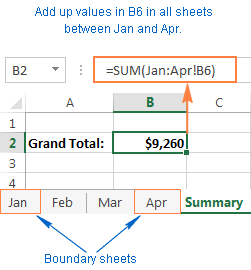
Tip. If you intend to copy your 3-D formula to several cells and you don't want the cell references to change, you can lock them by adding the $ sign, i.e. by using absolute cells references like =SUM(Jan:Apr!$B$6).
You don't even need to calculate a sub-total in each monthly sheet - include the range of cells to be calculated directly in your 3D formula:
=SUM(Jan:Apr!B2:B5)
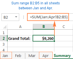
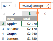
If you want to find out the sales total for each individual product, then make a summary table in which the items appear exactly in the same order as in monthly sheets, and input the following 3-D formula in the top-most cell, B2 in this example:
=SUM(Jan:Apr!B2)
Remember to use a relative cell reference with no $ sign, so the formula gets adjusted for other cells when copied down the column:
Based on the above examples, let's make a generic Excel's 3D reference and 3D formula.
Excel 3-D reference
First_sheet:Last_sheet!range
Excel 3-D formula
=Function(First_sheet:Last_sheet!range)
When using such 3-D formulas in Excel, all worksheets between First_sheet and Last_sheet are included in calculations.
Note. Not all Excel functions support 3D references, here is the complete list of functions that do.
How to create a 3-D reference in Excel
To make a formula with a 3D reference, perform the following steps:
- Click the cell where you want to enter your 3D formula.
- Type the equal sign (=), enter the function's name, and type an opening parenthesis, e.g. =SUM(
- Click the tab of the first worksheet that you want to include in a 3D reference.
- While holding the Shift key, click the tab of the last worksheet to be included in your 3D reference.
- Select the cell or range of cells that you want to calculate.
- Type the rest of the formula as usual.
- Press the Enter key to complete your Excel 3-D formula.
How to include a new sheet in an Excel 3D formula
3D references in Excel are extendable. What it means is that you can create a 3-D reference at some point, then insert a new worksheet, and move it into the range that your 3-D formula refers to. The following example provides full details.
Supposing it's only the beginning of the year and you have data for the first few months only. However, a new sheet is likely to be added each month and you'd want to have those new sheets included in your calculations as they are created.
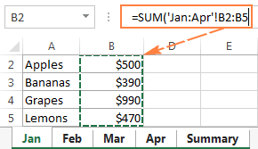
For this, create an empty sheet, say Dec, and make it the last sheet in your 3D reference:
=SUM(Jan:Dec!B2:B5)
When a new sheet is inserted in a workbook, simply move it anywhere between Jan and Dec:
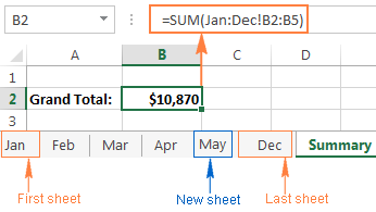
That's it! Because your SUM formula contains a 3-D reference, it will add up the supplied range of cells (B2:B5) in all the worksheets within the specified range of worksheet names (Jan:Dec!). Just remember that all of the sheets included in an Excel 3D reference should have the same data layout and the same data type.
How to create a name for an Excel 3-D reference
To make it even easier for you to use 3D formulas in Excel, you can create a defined name for your 3D reference.
- On the Formulas tab, go to the Defined Names group and click Define Name.
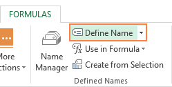
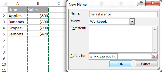
- In the New Name dialog, type some meaningful and easy-to remember name in the Name box, up to 255 characters in length. In this example, let it be something very simple, say my_reference.
- Delete the contents of the Refers to box, and then enter a 3D reference there in the following way:
- Type = (equal sign).
- Hold down Shift, click the tab of the first sheet you want to reference, and then click the last sheet.
- Select the cell or range of cells to be referenced. You can also reference an entire column by clicking the column letter on the sheet.
In this example, let's create an Excel 3D reference for the entire column B in sheets Jan through Apr. As the result, you'll get something like this:
- Click the OK button to save the newly created 3D reference name and close the dialog. Done!
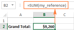
And now, to sum the numbers in column B in all the worksheets from Jan through Apr, you just use this simple formula:
=SUM(my_reference)
Excel functions supporting 3-D references
Here is a list of Excel functions that allow using 3-D references:
SUM - adds up numerical values.
AVERAGE - calculates arithmetic mean of numbers.
AVERAGEA - calculates arithmetic mean of values, including numbers, text and logicals.
COUNT - Counts cells with numbers.
COUNTA - Counts non-empty cells.
MAX - Returns the largest value.
MAXA - Returns the largest value, including text and logicals.
MIN - Finds the smallest value.
MINA - Finds the smallest value, including text and logicals.
PRODUCT - Multiplies numbers.
TEXTJOIN - combines values from multiple cells into one with a specified delimiter.
STDEV, STDEVA, STDEVP, STDEVPA - Calculate a sample deviation of a specified set of values.
VAR, VARA, VARP, VARPA - Returns a sample variance of a specified set of values.
How Excel 3-D references change when you insert, move or delete sheets
Because each 3D reference in Excel is defined by the starting and ending sheet, let's call them the 3-D reference endpoints, changing the endpoints changes the reference, and consequently changes your 3D formula. And now, let's see exactly what happens when you delete or move the 3-D reference endpoints, or insert, delete or move sheets within them.
Because nearly everything is easier to understand from an example, further explanations will be based on the following 3-D formula that we've created earlier:
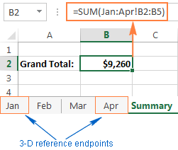
Insert, move or copy sheets within the endpoints. If you insert, copy or move worksheets between the 3D reference endpoints (Jan and Apr sheets in this example), the referenced range (cells B2 through B5) in all newly added sheets will be included in the calculations.
Delete sheets, or move sheets outside of the endpoints. When you delete any of the worksheets between the endpoints, or move sheets outside of the endpoints, such sheets are excluded from your 3D formula.
Move an endpoint. If you move either endpoint (Jan or Apr sheet, or both) to a new location within the same workbook, Excel will adjust your 3-D formula to include the new sheets that fall between the endpoints, and exclude those that have fallen out of the endpoints.
Reverse the endpoints. Reversing the Excel 3D reference endpoints results in changing one of the endpoint sheets. For example, if you move the starting sheet (Jan) after the ending sheet (Apr), the Jan sheet will be removed from the 3-D reference, which will change to Feb:Apr!B2:B5.
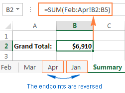
Moving the ending sheet (Apr) before the starting sheet (Jan) will have a similar effect. In this case, the Apr sheet will get excluded from the 3D reference that will change to Jan:Mar!B2:B5.
Please note that restoring the initial order of the endpoints won't restore the original 3D reference. In the above example, even if we move the Jan sheet back to the first position, the 3D reference will remain Feb:Apr!B2:B5, and you will have to edit it manually to include Jan in your calculations.
Delete an endpoint. When you delete one of the endpoint sheets, it is removed from the 3D reference, and the deleted endpoint changes in the following way:
- If the first sheet is deleted, the endpoint changes to the sheet that follows it. In this example, if the Jan sheet is deleted, the 3D reference changes to Feb:Apr!B2:B5.
- If the last sheet is deleted, the endpoint changes to the preceding sheet. In this example, if the Apr sheet is deleted, the 3D reference changes to Jan:Mar!B2:B5.
This is how you create and use 3-D references in Excel. As you see, it's a very convenient and fast way to calculate the same ranges in more than one sheet. While updating long formulas referencing different sheets might be tedious, an Excel 3-D formula requires updating just a couple of references, or you can simply insert new sheets between the 3D reference endpoints without changing the formula.
That's all for today. I thank you for reading and hope to see you on our blog next week!
 by
by
8 comments
When inserting a rows to all sheets in a 3D worksheet simultaneously, the formulas on the sheet accumulating data (call it SUM) from the other data sheets get misaligned. For instance, assume cell E11 on the SUM sheet originally summed all cell cells E11 on the rest of the sheets. If a new row 11 was inserted to all of the sheets, "data" in all cell E11's would shift down to cell E12. The formula in the SUM cell E12 now sums all the cells E11, which are blank on the other sheets. Several versions ago, they stayed aligned when rows or columns were added. I love 3D worksheets, but need a workaround to resolve this.
Hello!
Use absolute cell references or Defined name. I recommended this article.
what if I want to copy the value of the same range of cells (a2:h2 in the sheet tot gross) of different files in the same directory?
For example I have in the folder "september" 120 files named invoice1.xlms , invoice2.xlms , invoice3xlms.......invoice 120xlms.
I would like to create a new file who can copy the values I need that are in the same position in every file of the same folder.
Thanks for your help
Hello Alessandro,
Please try Consolidate Worksheets Wizard to see if it can help with your task.
Please use the link below to download and get additional details:
https://www.ablebits.com/excel-suite/combine-sheets.php
Just choose the options Copy the selected worksheets to one workbook and Paste link to data.
I was hoping this was the answer I'm looking for, but I don't think it is. Could you point me in the right direction?
In a Google AdWords Report, I have a sheet for each campaign I'm running. Each sheet has the same headings, and I would like them to have the same formulas. Google's Cost/Converted_Click formula is awful, because it doesn't assign a Cost if there is no converted click, although money is actually spent.
So I have a column for Cost and a column for Converted_Clicks. I would like to create named ranges for Cost and Converted_Clicks that refer to the same range on every sheet. Thus the formula =iferror(Cost/Converted_Clicks,Cost) would assign the cost even if the number of converted clicks is zero (div by zero error). On each sheet, that formula would refer to the cost and the converted clicks on that sheet.
Is this possible?
Hello Paul,
For us to be able to assist you better, please send us a small sample table with your data in Excel and include the expected result. Thank you.
I look to have a dynamic sheet name. meaning the sheet name in a SUM formula is from a cell where the name is created. any ideas??
Hello Gadi,
You can create a 3-D reference at some point, then insert a new worksheet, and move it into the range that your 3-D formula refers to.