The tutorial explains all main features of Excel conditional formatting with examples. You will learn how to do conditional formatting in any version of Excel, efficiently use preset rules or create new ones, edit, copy and clear formatting.
Excel conditional formatting is a really powerful feature when it comes to applying different formats to data that meets certain conditions. It can help you highlight the most important information in your spreadsheets and spot variances of cell values with a quick glance.
Many users, especially beginners, find it intricate and obscure. If you feel intimidated and uncomfortable with this feature, please don't! In fact, conditional formatting in Excel is very straightforward and easy to use, and you will make sure of this in just 5 minutes when you have finished reading this tutorial :)
What is conditional formatting in Excel?
Excel Conditional Formatting is used to apply certain formatting to data that meets one or more conditions. Just like usual cell formatting, it lets you highlight and differentiate your data in various ways by changing cells' fill color, font color, border styles, etc. The difference is that it is more flexible and dynamic - when the data changes, conditional formats get updated automatically to reflect the changes.
Conditional formatting can be applied to individual cells or entire rows based on the value of the formatted cell itself or another cell. To conditionally format your data, you can utilize preset rules such as Color Scales, Data Bars and Icon Sets or create custom rules where you define when and how the selected cells should be highlighted.

Where is conditional formatting in Excel?
In all versions of Excel 2010 through Excel 365, conditional formatting resides in the same place: Home tab > Styles group > Conditional formatting.
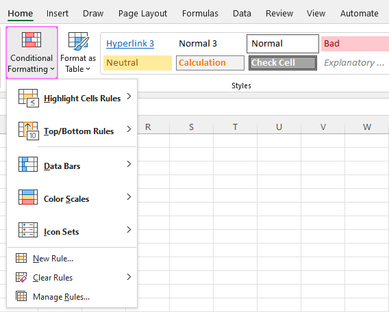
Now that you know where to find conditional formatting in Excel, let's move on and see how you can leverage it in your daily work to make more sense of the project you are currently working on.
For our examples, we will use Excel 365, which seems to be the most popular version these days. However, the options are essentially the same in all Excels, so you won't have any problems with following no matter what version is installed on your computer.
How to use conditional formatting in Excel
To truly leverage the capabilities of conditional format, you need to learn how to utilize various rule types. The good news is that whatever rule you are going to apply, it defines the two key things:
- What cells are covered by the rule.
- What condition should be met.
So, here's how you use Excel conditional formatting:
- In your spreadsheet, select the cells you want to format.
- On the Home tab, in the Styles group, click Conditional Formatting.
- From a set of inbuilt rules, choose the one that suits your purpose.
As an example, we are going to highlight values less than 0, so we click Highlight Cells Rules > Less Than…
- In the dialog window that appears, enter the value in the box on the left and choose the desired format from the drop-down list on the right (default is Light Red Fill with Dark Red Text).
When done, Excel will show you a preview of formatted data. If you are happy with the preview, click OK.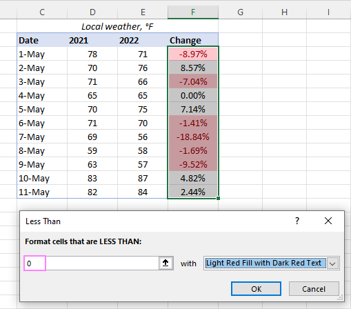
In a similar manner, you can use any other rule type that is more appropriate for your data, such as:
- Greater than or equal to
- Between two values
- Text that contains specific words or characters
- Date occurring in a certain range
- Duplicate values
- Top/bottom N numbers
How to use a preset rule with custom formatting
If none of the predefined formats suits you, you can choose any other colors for cells' background, font or borders. Here's how:
- In the preset rule dialog box, from the drop-down list on the right, pick Custom Format…

- In the Format Cells dialog window, switch between the Font, Border and Fill tabs to choose the desired font style, border style and background color, respectively. As you do this, you will immediately see a preview of the selected format. When done, click OK.

- Click OK one more time to close the previous dialog window and apply the custom formatting of your choice.

Tips:
- If you want more colors than the standard palette provides, click the More Colors… button on the Fill or Font tab.
- If you wish to apply a gradient background color, click the Fill Effects button on the Fill tab and choose the desired options.
How to create a new conditional formatting rule
If none of the preset rules meets your needs, you can create a new one from scratch. To get it done, follow these steps:
- Select the cells to be formatted and click Conditional Formatting > New Rule.

- In the New Formatting Rule dialog box that opens, select the rule type.
For example, to format cells with percent change less than 5% in either direction, we choose Format only cells that contain, and then configure the rule like shown in the screenshot below: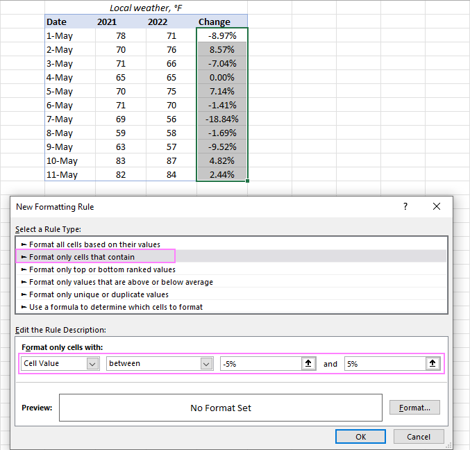
- Click the Format… button, and then choose the Fill or/and Font color you want.
- Click OK twice to close both dialog windows and your conditional formatting is done!

Excel conditional formatting based on another cell
In the previous examples, we highlighted cells based on "hardcoded" values. However, in some cases it makes more sense to base your condition on a value in another cell. The advantage of this approach is that irrespective of how the cell value changes in future, your formatting will adjust automatically to respond to the change.
As an example, let's highlight prices in column B that are greater than the threshold price in cell D2. To accomplish this, the steps are:
- Click Conditional formatting> Highlight Cells Rules > Greater Than…
- In the dialog box that pops up, place the cursor in the text box on the left (or click the Collapse Dialog icon), and select cell D2.
- When done, click OK.
As a result, all the prices higher than the value in D2 will get highlighted with the selected color:
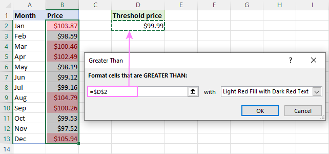
That is the simplest case of conditional formatting based on another cell. More complex scenarios may require the use of formulas. And you can find several examples of such formulas along with the step-by-step instructions here:
Apply multiple conditional formatting rules to same cells
When using conditional formats in Excel, you are not limited to only one rule per cell. You can apply as many rules as your business logic requires.
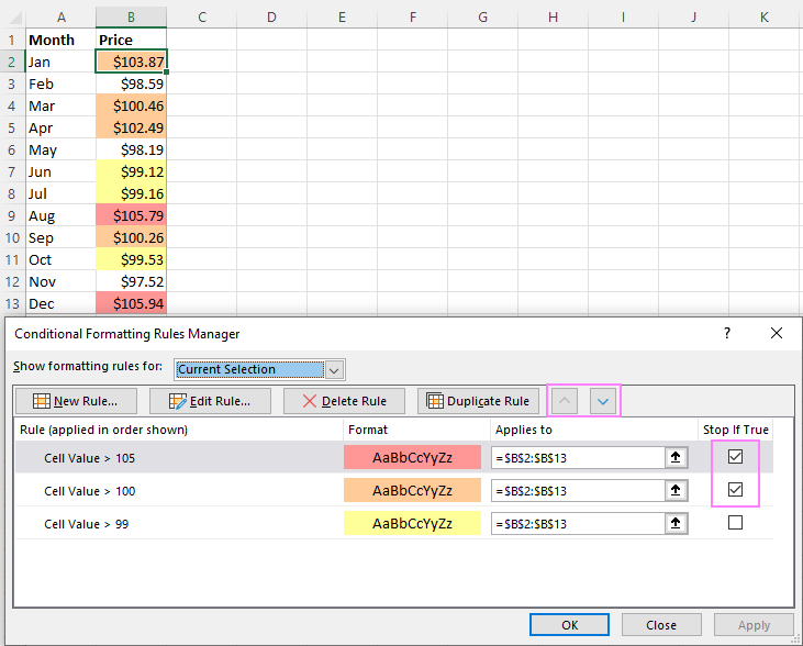
For example, you can create 3 rules to highlight prices higher than $105 in red, higher than $100 in orange, and higher than $99 in yellow. For the rules to work correctly, you need to arrange them in the right order. If the "greater than 99" rule is placed first, then only the yellow formatting will be applied because the other two rules won't have a chance to be triggered - obviously, any number that is higher than 100 or 105 is also higher than 99 :)
To re-arrange the rules, this is what you need to do:
- Select any cell in your dataset covered by the rules.
- Open the Rules Manager by clicking Conditional Formatting > Manage Rules…
- Click the rule that needs to be applied first, and then use the upward arrow to move it to top. Do the same for the second-in-priority rule.
- Select the Stop If True check box next to all but the last rule because you do not want the subsequent rules to be applied when the prior condition is met.
What is Stop if True in Excel conditional formatting?
The Stop If True option in conditional formatting prevents Excel from processing other rules when a condition in the current rule is met. In other words, if two or more rules are set for the same cell and Stop if True is enabled for the first rule, the subsequent rules are disregarded after the first rule is activated.
In the example above, we have already used this option to ignore subsequent rules when the first-in-priority rule applies. That usage is quite evident. And here are another couple of examples where the use of the Stop If True function is not so obvious but extremely helpful:
How to edit Excel conditional formatting rules
To make some changes to an existing rule, proceed in this way:
- Select any cell to which the rule applies and click Conditional Formatting > Manage Rules…
- In the Rules Manager dialog box, click the rule you want to modify, and then click the Edit Rule… button.
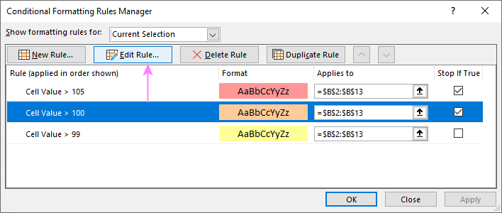
- In the Edit Formatting Rule dialog window, make the required changes and click OK to save the edits.
That dialog window looks very similar to the New Formatting Rule dialog box used for creating a new rule, so you won't have any difficulties with it.
Tip. If you don't see the rule you want to edit, then select This Worksheet from the Show formatting rules for drop-down list at the top of the Rules Manager dialog box. This will display the list of all the rules in your worksheet.
How to copy Excel conditional formatting
To apply a conditional format you've created earlier to other data, you won't need to re-create a similar rule from scratch. Simply use Format Painter to copy the existing conditional formatting rule(s) to another data set. Here's how:
- Click any cell with the formatting you want to copy.
- Click Home > Format Painter. This will change the mouse pointer to a paintbrush.
Tip. To copy the formatting to multiple non-contiguous cells or ranges, double-click Format Painter.
- To paste the copied formatting, click on the first cell and drag the paintbrush down to the last cell in the range you want to format.

- When done, press Esc to stop using the paintbrush.
- Select any cell in your new dataset, open the Rules Manager and check the copied rule(s).
Note. If the copied conditional formatting uses a formula, you may need to adjust cell references in the formula after copying the rule.
How to delete conditional formatting rules
I've saved the easiest part for last :) To delete a rule, you can either:
- Open the Conditional Formatting Rules Manager, select the rule and click the Delete Rule button.

- Select the range of cells, click Conditional Formatting > Clear Rules and choose the option that fits your needs.

This is how you do conditional formatting in Excel. Hopefully, these very simple rules we created were helpful to get a grasp of the basics. Below, you can find a few more tutorials that can help you understand the inner mechanics and expand conditional formatting in your spreadsheets far beyond its traditional uses.
Practice workbook for download
Excel conditional formatting - examples (.xlsx file)
 by
by
314 comments
Dear Developer, Often I use conditional formatting at my Excel spreadsheets, however the condition (color) used to explain the reason of a cell or a range, can differ based on the designer and the user of the product/workbook, in this case I have to first train the user, that why I had put that condition to get particular color, Here it is difficult for one to use the spreadsheet without explanation, is there way; where I can put my text Explaining the reasoning?
Or suggest to add a text field at conditional module to add user thought.so that user can read the reasoning why this condition has been inserted/used
E.g. We all Universally know that RED means Danger, Yellow means be alert or, Green means OK, but it may differ based on the user prospective, if he does not know what the RED stand for, or Green is OK or v/versa
In my case color Blue can stand for RED
Please let me know
Happy New Year 2016
hello, pls am trying to use a colour code for excel i want to use a data in one column to change the row colour based on the input on any other column like i have a 7 in column b and want it to change to a colour red when i input D in any other column
Hello,
Though you can't create a rule for all columns, you can try listing certain columns that the rule will check. E.g. select column A and create a rule with the following formula:
=OR($B1="D",$C1="D",$D1="D",$E1="D",$F1="D",$G1="D")
If any of the listed cells contain "D", it will highlight the cell in column A.
First- I want to thank you for all the great tips. I am creating a workbook that has 6 tabs (goals) - each tab containing the goals for a particular metric for a particular region. Each tab is identical in set up but has different values for the goals. I also have 6 tabs with each regions report card. On those tabs i enter the actual result for a metric and use conditional formatting to look at the value to the goals tab for that particular region. If i create one report card i want to be able to copy it 5 times. My problem is the conditional fomatting will still look at the conditional formatting for the first one i created and look at the 1st goal tab. I want to be able to copy the original worksheet but want a quick way to change the worksheet reference in all conditional formatting formulas for a particular worksheet- can this be done?
Hello Karen,
When you copy the conditional formatting rule, you need to change the worksheet name; please also make sure you use relative references for your rules.
You can find more information about absolute and relative references in this blog post:
https://www.ablebits.com/office-addins-blog/relative-absolute-cell-references-excel-conditional-formatting/
I want to compare one column A of Catalog Numbers containing lot numbers in column B to one column C of Catalog Numbers containing lot numbers in column D and populate the items that match in column E as 0 and the items that don't match in column E as-1 and highlighted in red,
Hello,
If we understand your task correctly and you are trying to compare the lot numbers in column D to lot numbers in column B, then enter the following formula into E1:
=IF($D1=$B1,0,-1)
Copy it down the entire column to get the results for all rows.
Then create a conditional formatting rule with the formula below to highlight those cells in column E that contain "-1":
=$E1=-1
Hi,
I have two rows, the first one with various targets/thresholds and the second onwards with achieved values. While I apply the conditional formatting it gets applied to the entire table. Since the targets are different for each row, I could not do it by just formatting the first row and pasting the format for the rest. There should be a work around which I'm not aware. Please help.
Hello Karthik,
Most likely there is an issue with absolute and relative references in the formula you use for the conditional formatting rule. You can add a dollar sign before the row or column reference to make sure it is not changed. Please see this blog post for a detailed description of using relative and absolute references in your conditional formatting rules:
https://www.ablebits.com/office-addins-blog/relative-absolute-cell-references-excel-conditional-formatting/
Thank you so much for the reply Irina. Your solution helped me a lot of time.
I need help in inserting specific comment based on the value of certain cell. E.g.: If the value of cell A1 is greater than equal to 3 then I would like to generate a comment in B1 stating 'reporting not required', so as A1=4, comment in B1 should read as 'reporting required' and so on for different values in A1. Is this possible in Excel? Appreciate your guidance.
Hello Shiv,
You can add the following formula to cell B1 and copy it down the column:
=IF(ISBLANK($A1),"",IF($A1<=3,"reporting not required",IF($A1=4,"reporting required","new rule")))
Hello,
Whether can we autocapture the formatted text such as (B,U,L) and replace with some html tags.
Can i know how to write it.
Regards,
Navaneeth
Hi,
WHAT FORMULA TO USE TO FILL UP THE CELL,THANKS
SHIPREFT COUNTRY SHIP MODE
JTWA555666 ? ?
JSYS2555333 ? ?
JBKT555999 ? ?
Ship COUNTRY SHIP MODE
JSYS Australia SEA
JTWA TAIWAN AIR
JBKT THAILAND TRUCK
Hello Lisa,
You need to use the VLOOKUP function for your task. Here is the formula you need to enter in the "Country" column:
=VLOOKUP(LEFT(A16,4),Sheet2!A1:C4,2,FALSE)
It looks at the first four characters in cell A16 (your SHIPREFT), compares them to the value in the first column in Sheet2!A1:C4, and returns the corresponding value from the second column in that range.
You can learn more about the VLOOKUP function in this blog post:
https://www.ablebits.com/office-addins-blog/excel-vlookup-tutorial/
Hi, is it possible to create a rule to give a value to a work.
For example: I have a checklist and from a drop down list I can select a number of words, Conformance, Non-conformance and Partial non-conformance, now I would like to automatically have a value assigned to each of these in another column.
i.e. Conformance = 3; Partial non-conformance = 2 and non-conformance = 0.
How would I do this.
Hello Lizl,
You can enter the following formula into the cell where you want to get the value:
=IF(F2="Conformance",3,IF(F2="Non-conformance",0,IF(F2="Partial non-conformance",2,"")))
Here F2 is the cell with the drop-down list.
hi anybody can provide me excel data for practise.
Hello,
You can use our Random Generator add-in to create sets of data for practice:
https://www.ablebits.com/excel-random-generator/index.php
Need to lock conditional formatting but still allow values to be pasted into those formatted cells from other sources.
Problem: I have set up a spreadsheet that highlights cells that need to be populated or left blank. Certain cells that need to be populated are highlighted based on a particular part type (which is chosen from a dropdown menu for the cells located in column AF). Since we are looking over data that can be up to 2000 thousand rows and covering columns A-CL it would take hours to retype all the information to ensure the right columns are populated based on that part type. It is easier to just paste the values in from outside sources. However, it would make it easier to audit the data if the highlighted cells remained highlighted after those values are pasted in.
Question: Is there a way to lock the formatting while at the same time allowing those conditionally formatted cells (that are highlighted) to have values pasted as an overlay from other sources without deleting the format?
Thanks,
Hello Aaron,
Unfortunately you can't keep conditional format using the standard means of Excel. You may be able to do this with the help of VBA, please try posting your question on the VBA branches of the following websites: https://www.excelforum.com/ or https://www.mrexcel.com/
Great Svetlana Cheusheva,
Hope you will be fine.
Today I did my best to solve one of my problems regarding conditional formatting and at last when I read your guidelines and instructions step by step. So these procedures were really easy and were found satisfactory and would like to say special thanks & regards to your efforts and technical support to the needy individuals who are facing problems in MS excel.
Once again thanks
Regards,
Cadet Dani
Hi
I have two documents in word containing employee's names but one document starts people's names like Yusuf Mariam and the other Mariam Yusuf so it's confusing me wheather it's one person's name or two people with different names.Please help me with the format i can use to identify them in excel 2013.
Hi
How do i copy the colour in a formatted cell to a name cell?
Thanks
Is there any way to use conditional formatting to show cells that have been edited? I cannot use Track Changes because I do not want to convert my table to range.
If not conditional formatting, is there any other way to do this?
Hello Shannon,
Conditional formatting can't do this, you need a VBA macro. If you don't need to keep the changes after you close the workbook, you can use the code below:
- Open your Excel file and press Alt+F11 on your keyboard;
- Select the necessary sheet in the list and paste this code:
Private Sub Worksheet_Change(ByVal rnUpdated As Range)
rnUpdated.Interior.Color = CLng("&H00FF00")
End Sub
I WANT TO KNOW THAT HOW CAN I GET THE HIGHLIGHTED CELL FOR TOP 5 PERSON'S NAME ON THE BASE OF ORDER... EX:-
CUSTOMER NAME ORDER QUANTITY
JOHN LARSON 120
FRANCIS MONTGOMERY 126
JENNA SAIZ 67
KELLY PICKETT 98
MARIA HERNANDEZ 111
HUGO LAWS 210
RICHARD BAKER 106
JOEL CANO 130
STEVE TAYLER 36
PLZ.. GIVE A SOLUTION FOR THIS IN A EASILY UNDERSTANDABLE WAY.. THANX IN ADVANCE...
good day
excel 2010,
conditional formatting rules manager
new rule
format only cells that contains
format only cells with
cells value
equal to:4 and 5 and 10 and 17 and 35 etc..in the same line
(not equal to:4
then
equal to 5
equal to 10 in different lines
all those numbers in one line)
then format
fill
and so on
is it possible in excel 2010 or 2013.
thanks
Halevy yosef
Hi, I am trying to create a conditional format the when Cell B2 = or contains a certain word then a particular number goes into cell C2, D2 or E2 depending on what Cell B2 contains.
ie if B2 = cat then C2 = 1, if B2 = dog then C2 = 1 and D2 = 1 etc
Thanks in advance
Hi Jurgen,
With conditional formatting you can only "format" cells, i.e. change their background or font color, add icon sets or color scales, etc.
To put a certain value in a cell depending on another cell's value, you need an IF formula. For example:
Formula for C2: =IF(OR(B2="cat", B2="dog"), 1, "")
Formula for D2: =IF(B2="dog", 1, "")
Hi can you help me with this problem?
I want to separate the amount in an excel 2007
For example:
A1 = 12
I want the answer would be
A2 = 5 (Constant/or Keeps the value Lesser or equal to 5 but not negative)
A3 = the excess amount from the value of A1
Hi Kimoy,
If my understanding of your task is correct, you can simply put 5 (or any other number you want) in A2, and =A1-A2 in A3.
Hello, I am trying to do conditional formatting on a finacial scorecard. I need to do Red, Yellow Green based on the following criteria.
Column B is my target revenue - $30,000 - Every column after that is for a week of revenue and I need to color them based on the following guidelines.
Within 5% - Green
Within 5-10% - Yellow
More then 10% - Red
So if Column D's revenue is $45,000, I need to color it Red. But if column E's revenue is $30,500 it should be green.
I have tried everything and I am sure I am making a silly mistake. Can you please help?
Thanks!
Hey Tina,
I don't know if you're still having this issue, but this may be helpful to other users if you've already figured it out!
Assuming the following:
- The first target revenue is in B1 (if not, simply adjust the formulas used below)
- The first week's revenue is in C1 (same note as above)
You can do the following to accomplish your goal:
(With C1 selected)
We need to make three rules, one for each case. All of the following rules will be added using the following process:
1. Click the "HOME" tab on the menu bar
2. Click "Conditional Formatting"
3. Click "New Rule..."
4. Click "Use a formula to determine which cells to format"
### For red: ###
Assure that C1 is selected!
1. Begin adding a new rule (using the process above)
2. Paste the following formula in the formula text box:
=OR(C1$B1*0.1)
3. Click “Format…” and set the fill color to red
4. Personally I set the font color to white to make it more readable, but this isn’t necessary
5. Click “OK”, you’re done!
Now when the revenue in C1 is outside a 10% margin of the target revenue, the cell will be filled red! (Note that blank cells will also be filled red, this is covered in the section “Catching blank cells”)
### For yellow (very similar to process for red): ###
Assure that C1 is selected!
1. Begin adding a new rule (using the process above)
2. Paste the following formula in the formula text box:
=AND(C1>=$B1-$B1*0.1, C1=($B1-$B1*0.05),C1<=$B1*1.05)
3. Click “Format…” and set the fill color to green
4. Click “OK”, you’re done!
Now when the revenue in C1 is within a 5% margin of the target revenue, the cell will be filled green (be sure to check out the “IMPORTANT” section to make sure this works)!
### Catching blank cells: ###
Assure that C1 is selected!
You can skip the next section if you want blank cells to be filled red (or don’t mind either way)
1. Begin adding a new rule (using the process above)
2. Paste the following formula in the formula text box:
=ISBLANK(C1)
3. Click “OK”, you’re done!
Now blank cells will simply be ignored!
### IMPORTANT!! ###
To assure that the rules act as intended please do the following:
1. Click “Conditional Formatting”
2. Click “Manage Rules…”
3. Make sure that the rules are in the following order (distinguishable by the fill color):
Blank
Green
Yellow
Red
NOTE: Rules can be moved up or down using the arrow buttons to the right of "Delete Rule"
4. Make sure that for each rule the “Stop If True” box is checked (far right column)
This assures that only one rule will be applied to any given cell
### Finishing up: ###
Now that we have all the rules made for C1, we want to be able to apply the same rules to other cells!
The process for copying conditional formatting is included in the main article, but the process is summarized below:
1. Select C1
2. Click “Formula Painter” under the “HOME” tab
3. Drag from C1 to the end of the range of cells you wish to copy the formatting to (e.g. from C1 to L1 or from C1 to C10 or from C1 to L10)
That’s it! Please let me know if you (or anyone else reading this) experience any problems!