The tutorial explains how to write formulas in Excel, beginning with very simple ones. You will learn how to create a formula in Excel using constants, cell references and defined names. Also, you will see how to make formulas using the function wizard or enter a function directly in a cell.
In the previous article we've started to explore a fascinating word of Microsoft Excel formulas. Why fascinating? Because Excel provides formulas for almost anything. So, whatever problem or a challenge you are facing, chances are that it can be solved by using a formula. You just need to know how to make a proper one :) And it is exactly what we are going to discuss in this tutorial.
For starters, any Excel formula begins with the equal sign (=). So, whatever formula you are going to write, begin by typing = either in the destination cell or in the Excel formula bar. And now, let's have a closer look at how you can make different formulas in Excel.
How to make a simple Excel formula by using constants and operators
In Microsoft Excel formulas, constants are numbers, dates or text values that you enter directly in a formula. To create a simple Excel formula using constants, just do the following:
- Select a cell where you want to output the result.
- Type the equal symbol (=), and then type the equation you want to calculate.
- Press the Enter key to complete your formula. Done!
Here is an example of a simple subtraction formula in Excel:
=100-50
How to write formulas in Excel using cell references
Instead of entering values directly in your Excel formula, you can refer to the cells, containing those values.
For example, if you want to subtract a value in cell B2 from the value in cell A2, you write the following subtraction formula: =A2-B2
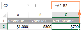
When making such a formula, you can type the cell references directly in the formula, or click the cell and Excel will insert a corresponding cell reference in your formula. To add range reference, select the range of cells in the sheet.

Note. By default, Excel adds relative cell references. To switch to another reference type, press the F4 key.
A big advantage of using cell references in Excel formulas is that whenever you change a value in the referred cell, the formula recalculates automatically without you having to manually update all the calculations and formulas on your spreadsheet.
How to create an Excel formula by using defined names
To take a step further, you can create a name for a certain cell or a range of cells, and then refer to that cell(s) in your Excel formulas by simply typing the name.
The fastest way to create a name in Excel, is to select a cell(s) and type the name directly in the Name Box. For example, this is how you create a name for cell A2:

A professional-like way to define a name is via the Formulas tab > Defined names group or Ctrl+F3 shortcut. For the details steps, please see creating a defined name in Excel.
In this example, I've created the following 2 names:
- revenue for cell A2
- expenses for cell B2
And now, to calculate the net income, you can type the following formula in any cell on any sheet within the workbook in which those names were created: =revenue-expenses
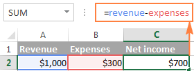
In the same manner, you can use names instead of cell or range references in arguments of Excel functions.
For example, if you create the name 2015_sales for cells A2:A100, you can find a total of those cells by using the following SUM formula: =SUM(2015_sales)
Of course, you can get the same result by supplying the range to the SUM function: =SUM(A2:A100)
However, defined names make Excel formulas more understandable. Also, they can significantly expedite creating formulas in Excel especially when you are using the same range of cells in multiple formulas. Instead of navigating between different spreadsheets to find and select the range, you just type its name directly in the formula.
How to make Excel formulas by using functions
Excel functions are nothing else than predefined formulas that perform the required calculations behind the scene.
Each formula begins with an equal sign (=), followed by the function name and the function arguments entered within the parentheses. Each function has specific arguments and syntax (particular order of arguments).
For more information, please see a list of the most popular Excel functions with formula examples and screenshots.
In your Excel spreadsheets, you can create a function-based formula in 2 ways:
Create a formula in Excel by using the Function Wizard
If you do not feel very comfortable with Excel spreadsheet formulas yet, the Insert Function wizard will give you a helpful hand.
1. Run the function wizard.
To run the wizard, click the Insert Function button on the Formulas tab > Function Library group, or pick a function from one of the categories:
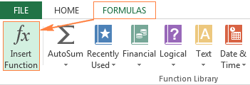
Alternatively, you can click the Insert Function button ![]() to the left of the formula bar.
to the left of the formula bar.
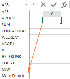
Or, type the equal sign (=) in a cell and pick a function from the drop-down menu to the left of the formula bar. By default, the drop-down menu displays 10 most recently used functions, to get to the full list, click More Functions...
2. Find the function you want to use.
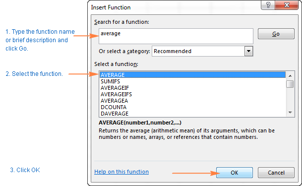
When the Insert Function wizard appears, you do the following:
- If you know the function name, type it in the Search for a function field and click Go.
- If you are not sure exactly what function you need to use, type a very brief description of the task you want to solve in the Search for a function field, and click Go. For example, you can type something like this: "sum cells", or "count empty cells".
- If you know what category the function belongs to, click the small black arrow next to Select a category and choose one of the 13 categories listed there. The functions belonging to the selected category will appear in the Select a function
You can read a short description of the selected function right under the Select a function box. If you need further details regarding that function, click the Help on this function link near the bottom of the dialog box.
Once you've found the function you wish to use, select it and click OK.
3. Specify the function arguments.
In the second step of the Excel function wizard, you are to specify the function's arguments. Good news is that no knowledge of the function's syntax is required. You just enter the cell or range references in the arguments' boxes and the wizard will take care of the rest.
To enter an argument, you can either type a cell reference or range directly into the box. Alternatively, click the range selection icon next to the argument (or simply put the cursor into the argument's box), and then select a cell or a range of cells in the worksheet using the mouse. While doing this, the function wizard will shrink to a narrow range selection window. When you release the mouse button, the dialog box will be restored to its full size.
A short explanation for the currently selected argument is displayed right under the function's description. For more details, click the Help on this function link near the bottom.
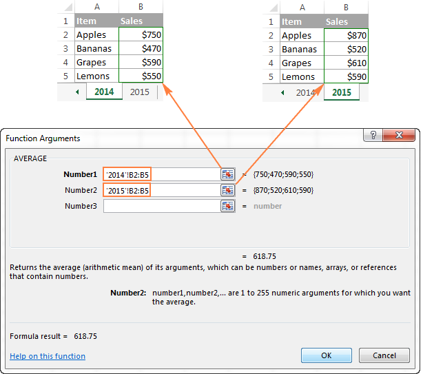
Excel functions allow you to perform calculations with cell residing on the same worksheet, different sheets and even different workbooks. In this example, we are calculating the average of sales for 2014 and 2015 years located in two different spreadsheets, which in why the range references in the above screenshot include the sheet names. Find more about how to reference another sheet or workbook in Excel.
As soon as you've specified an argument, the value or array of values in the selected cell(s) will be displayed right to the argument's box.
4. Complete the formula.
When you have specified all the arguments, click the OK button (or just press the Enter key), and the completed formula is entered into the cell.

Write a formula directly in a cell or formula bar
As you've just seen, creating a formula in Excel by using the function wizard is easy, thought it's quite a long multi-step process. When you have some experience with Excel formulas, you might like a faster way - typing a function directly into a cell or formula bar.
As usual, you start by typing the equal sign (=) followed by the function name. As you do this, Excel will perform some kind of incremental search and display a list of functions that match the part of the function's name you've already typed:
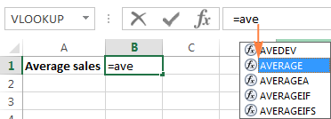
So, you can either finish typing the function name on your own or select from the displayed list. Either way, as soon as you type an opening parenthesis, Excel will show the function screen tip highlighting the argument you need to enter next. You can type the argument in the formula manually, or click a cell (select a range) in the sheet and have a corresponding cell or range reference added to the argument.
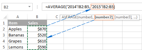
After you've input the last argument, type the closing parenthesis and hit Enter to complete the formula.
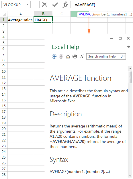
Tip. If you are not quite familiar with the function's syntax, click the function name and the Excel Help topic will pop-up right away.
This is how you create formulas in Excel. Nothing difficult at all, is it? In the next few articles, we will continue our journey in the intriguing realm of Microsoft Excel formulas, but those are going to be short tips to make your work with Excel formulas more efficient and productive. Please stay tuned!
 by
by
42 comments
how to calculate the ifs formular
Hi! I recommend reading this guide: Use Excel IFS function instead of nested IF
I've been trying to enter a formula into a worksheet tab and I can't get it to work. Is it even possible to do? I'm wanting the tab to show the current day's date (for ex. it would have 8.13.24 if I opened it today and then tomorrow if i opened it then it would say 8.14.24.
Thanks for any help and guidance.
Thanks!
Hello Myra!
If I understand the question correctly, you want to automatically rename a worksheet. This cannot be done using an Excel formula, but it is possible with VBA. If you want to insert the current date into a cell, use this instruction: Excel TODAY function to insert today's date.
if i insert some data in A1 cell today, and that data will automatically display on another A3 cell and next day i insert some data in A1 cell in this place i need to display in cell A3 Both First Day Data and Second Day Data it self , Kinddly Suggest Some Idea
Hi!
A cell can contain only one value. Or use a VBA macro to combine the old and new values of an A3 cell into one text string.
Hi, i have a question. The above post says about the existing formulas in Excel.
In Excel 2021, there is custom formula option using java script and saving the file.
Is there any way to insert custom formula in MS Excel 2016.
For example, I require numbers to be presented in Text as well
Cell A1: 2000
Cell A2: Two Thousand
There is option for the same in 2021 version of MS Excel "=Spellnumber" but, how to do the same in 2016 version, without VBA and macro enabled workbook, to be specific
Hi!
If I understand correctly, we have a special tutorial on this. Please see - Two best ways to convert numbers to words in Excel
I hope it’ll be helpful.
I need a formula,
Eg
Customer name Achieve QTY Basic value
A 5 150
B 5 150
A 5 150
C 15 450
B 5 150
A 5 150
this is the details here i need to take customer name "A" first "10" basic value.
Result
A 5+5 150+150
A 10 300
like this
any one can help me.
Hello, if you haven't yet got answer for your question... Use a =SUMIF formula. It gives you options for the above.
Hello, i am working on an excel sheet i need help
I want to know who are taking medicine in a village
I fill a table column by the name of the villagers and another by medicine and the 3rd is insurence
The medicine and indusrence column only include yes or no
How could i make on another page only the name of the villager display automatically if he takes medicine and doesn't have insurence?
Thank you for your help
Hello!
I think this article will be useful to you - How to VLOOKUP multiple values in Excel with one or multiple criteria
(2+2)/2*2 =?
4 :)
i need a formula
if "A2" value >100 then (*"C2") other then (*"A2*C2/100")
Hello Himanshu,
Please try the formula below to solve your task:
=IF(A2>100,B2*C2,B2*A2*C2/100)
Hi I need help
I would like to split 1.5x 2.5 which is in the same column.
I want data to be in different column or seperated to be
1.5
2.5
How can I do that
Hi Madilin,
Thank you for contacting us.
If we understand your task correctly, please have a look at our Split Cells tool. It can help you separate your text into multiple columns or rows at a glance.
I am trying to find a formula to figure out 6% sales tax.
Sales ÷tax = expenses
Thank you
Carley:
I think what you want is the formula:
=sales cell address/.06
I am trying to write the following formula in excel
x=100[((4a+b+c+d)e)-6]/254 where a, b, c, d, e have numerical values in various cells.
Can some help !
Many thanks
Mushtak:
I think this will provide the result you're after:
=100*(((4*(A1)+B1+C1+D1)*E1)-6)/254
Note the A1, B1, C1, D1 and E1 are cell addresses that you can modify.
Note the asterisk Excel uses to signify multiply.
Note there are no square brackets.
if i want that no.enter in the cell should be divided by 1000 and round upto one decimal place. like 6145 should be converted into 6.1
what will be the formula .
Virendra:
The simplest way to get what you want is to apply some arithmetic and then formatting a cell as a number to display one digit. If you want to do this "automatically" you'll need to build some VBA code and that's beyond the scope of this blog. I'll show you the easy method.
Let's say your number is in cell A2. Maybe it is 6145.
First, in cell B2 enter =A2/1000.
Next you'll format the cell B2 as a number with one decimal place.
To format the cell, right click on B2, choose Format Cells, then choose Number, then select 1 decimal place. Click OK.
The number displayed is "6.1".
Some arithmetic, some formatting and you're home.
Sales Person Margin A B C
A 50 50
B 100 100
C 120 120
A 110 110
A 50 50
a 60 60
B 70 70
B 20 20
above table shows some Values i need automatically insert margins I column A, B and C
Use text to columns function in the excel.
Irina,
Please help me with a formula
(1) If a cell value is less than or equals to 15000 then its 12% should be calculated.
(2) If the cell value is greater than 15000 then no calculation should happen.
Regards
Hello Viswanath,
Assuming that your values are in column E, here is the formula you need:
=IF($E2<=15000,($E2*12%),$E2)
I have a list of names that I want to match on another list. If it matches, I want it to enter a value in a cell. Example: I have a list of 50 names on one list. On the other I have another list of names with a column showing what group they are in (1, 2, 3 etc). I want to put a column next to the first list of names title group. I want the formula to go to the other list, find the name and enter the correct group number. Help?
Hello Trudee,
You need to use the VLOOKUP function. If we assume that the names are in column A, this is the formula you need:
=IFERROR(VLOOKUP($A2,Sheet2!A2:B12, 2, FALSE),"")
It compares the name in column A to the name in column A of Sheet2, and returns the corresponding group from the second column in Sheet2.
You can find a detailed description of the VLOOKUP function in this blog post:
https://www.ablebits.com/office-addins-blog/excel-vlookup-tutorial/
Dear Mam,
I have a issue of multiple line item of excel and want to make merge with the word document and also want to produce as a result which it should dispense to the single page of word document.
awaiting for your reply.
Thanks & Regards,
ashish Kumar mahapatra
Cell:+91-9437212127
Dear Ashish,
Integration of Excel with other applications can be done only with the help of VBA code.
Hey ,
When u type the formula =5! Y can’t we get the factorial y do we have to use the Fact function
Also how do u use # operator in formula
Hi Svetlana,
Thank you very much for providing the link. I went trough whole formulas in the provided link, they are really helpful I really appreciate it but the formula I need is a little more complicated.
Suppose we have 1000 villages and we give a single unique ID to each village, for example: The given unique ID for "Village1" is "0001", Unique ID for "village2" is "0002",... and Unique ID for "village1000" is "1000". Then we type the formula that if in column A1 I put the Unique ID "0001", in column B1 "Village1" should appear automatically and if I put the unique ID "0002" in column A2, in column B2 "Village2" should appear... and finally if I put the unique ID "1000" in Column A3, "Village1000" should appear in column B3.
I have the list of all those 1000 villages and giving and ID is simple but the only problem is the formula that if we use =If formula for the mentioned purpose, we will need to type each 1000 villages with their Unique IDs, that will take to much time and there is a big possibility of more mistakes for typing such a long formula, so do we have a simpler formula for the mentioned purpose?
And thank you very much, you really do a great job and please keep it on :).
Hi Suliman,
The IF function is not quite suitable for this task. What you need is a VLOOKUP formula that can search for a given ID (lookup value) across the ID's list and return a match from another column (village).
Just be very careful when assigning ids like "0001". Excel cuts off leading zeros in numbers and this may cause problems.
hello mam! do you know a formula for: enter cash total, result (cash pieces of denominations and denomination multiplied to pieces). Looking forward to your positive response. thank you!
I want to schedule tasks/ chores (6) for my kids (5) is there any ease way to do this with a formal. Jake does chore 1 for 5 days and gets 2 days off etc; maddie does a chore for 6 days and get 3 days off and then the awful chore (bathrooms) just rotates through the kids . They key is to be FAIR
Is there a formal I can use- to remove the kids thinking a love one more than the other
Sorry, I cannot think of any formula that could do this. My first thought was using the RANDBEETWEEN function. Something like assigning a certain number to each chore, and then using a RANDBEETWEEN formula to pick up random numbers for each kid. Upon a second thought, however, this does not look like a good idea. The assigned chores would be random, but not evenly distributed. Really sorry for not being able to help with your task :(
Hi Svetlana,
Thanks for your contribution on Excel. It is amazing. I used the dynamic data validation process mentioned by you. Keep up the good work.
Thank you Deepanshu! I'm glad my articles have helped in your work.
Hello,
I am a type of person who is always starving to learn something new of excel tricks and formulas.
I searched a lot in Google but couldn't find the formula I am seeking. I had seen a finance voucher document that a kind of formula was used in, that suppose Different Cash Books, Vehicle Fuel and at last everything had a unique code. The formula was set in a way that if we put the unique code for Vehicle Fuel in cell no "C2", the text "Vehicle Fuel" will automatically appear in cell no "B2". A short example is added in below:
C2 | C3
USD Cash Book | 10010001
EURO Cash Book | 10010002
Vehicle Fuel | 10050001
Is there a way to have an overview or get the lessons of the formula to how to use it? It will be much appreciated.
Thanks,
Suliman
Hi Suliman,
It looks like we have one thing in common. Like you, I also strive to learn something new every day :)
As for the formula you described, it seems to be an IF function that checks for blank/non-blank cells, for example:
=IF(C2<>"", "Vehicle Fuel", "")
The formula reads as follows: if cell C2 is not empty, return the text "Vehicle Fuel", otherwise return an empty string (blank cell).
For more IF formula examples, please see:
https://www.ablebits.com/office-addins-blog/if-function-excel/