 by
by See how you can create custom rules to color your data by any conditions.
Conditional formatting based on another cell: video transcript
There is no doubt that conditional formatting is one of the most useful features in Excel. Standard rules let you quickly color the necessary values, but what if you want to format entire rows based on a value in a certain cell? Let me show you how you can use formulas to create any conditional formatting rule you like.
Apply conditional formatting if another cell is blank
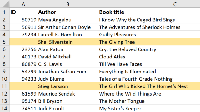
Here is one common task: I want to highlight the rows with a blank ID. Let's begin with the steps for creating a custom rule:
- First of all, select the range that you want to highlight, this will save you some steps later. Make sure you start with the top-left record and omit the header row. Converting the range to a Table is a better option if you plan to apply the rule to new entries in the future.
- Click on Conditional formatting at the top and choose "New rule". You need the last item: "Use a formula to determine which cells to format".
- Now you can enter your custom condition and set the desired format.
- A fill color offers the quickest way to see our data, so let's pick one and click ok.
- The formula to find the rows with blanks in column A is
=A2="". But that's not all. To make sure the rule is applied row by row, you need to make the reference to the column absolute, so enter a dollar sign before column A:=$A2=""If you wanted to always look at this particular cell, then you'd fix the row as well, making it look this way: $A$2=""
- Click Ok and here you go.
Excel conditional formatting based on another cell value
Now let's move on and see how we can find those book titles that have 10 or more in column E. I'll go ahead and select the book titles because this is what we want to format, and create a new Conditional Formatting rule that uses a formula. Our condition is going to be similar:
=$E2>=10
Pick the format and save the rule to see how it works.
As you can see, these are simple rules where you can enter any value that interests you. Where the value is, is not important. If it's in a different sheet, then simply make sure you include its name into your reference.
Conditional formatting formula for multiple conditions
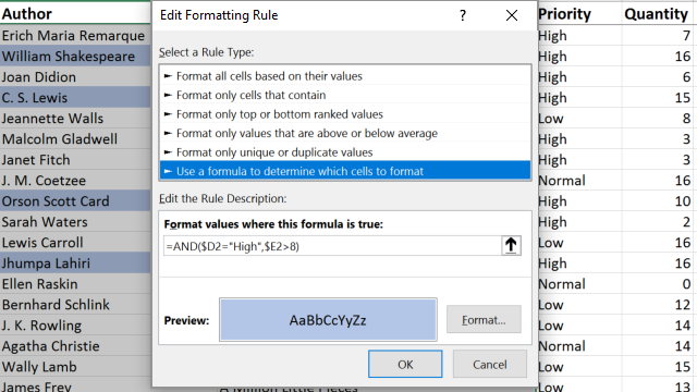
Let's move on to the cases when your condition concerns two different values. For example, you may want to see the orders that have a high priority and over 8 in the quantity field.
To change an existing rule, pick Manage rules under Conditional formatting, find the rule and click Edit. To make sure several conditions are met, use function "AND", then list your criteria in brackets and remember to use quotes for text values:
=AND($D2="High",$E2>8)
If you want to make sure at least one condition is met, then use OR function instead. Replace the function, now it will read: highlight the row if the priority is high or if quantity is over 8.
Formatting based on another cell text
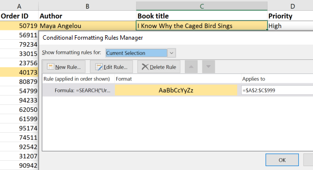
Here is another function you will appreciate if you work with text values. The task will seem tricky if you want to look at the cells that contain the key word along with anything else. If this is your case, you will need to use the Search function, and here is how it will look. Select the records to color, create a rule, and enter:
=SEARCH("Urgent",$F2)>0
Note that If you enter more than 1, then you'll get the cells that start with this text instead.
Things to remember for your custom rules
You can use practically any formula as a condition for highlighting your data. In one of our previous videos, we covered how to identify duplicates with the help of Conditional Formatting, and you can find some more great formula examples in our blog post on this topic.
Before you go formatting your table, let me quickly go over some typical mistakes that may not let you get the results you expect.
First of all, remember about the difference between absolute and relative cell references. If you want to check each cell in a column, enter a dollar sign before the name of the column. To keep checking the same row, add the dollar sign before the row number. And to fix the cell reference, in other words, to keep checking the same cell, make sure you have a dollar sign before both: the column and the row.
Then, if you see that your rule is applied just to one row or cell, go back to Manage rules and make sure it applies to the correct range.
When you create a rule, always use the top-left cell of the range with your data for the formula and omit the header row to avoid shifting the results.
As long as you keep these points in mind, Conditional Formatting formulas will do wonders to your data. If you still have troubles getting it to work for you, please share your task in comments, we'll do our best to help you.
79 comments
I am trying to write a permit for work for my job, what i am wanting to do is when a certain drop down box is changed I require that to change the colour in a merged cell I have made with the company name in it, oink for hot work(naked flame), yellow for hot work (spark potential), blue for cold work.
I can change the colour of the drop down box with no issues but, I just cant seem to figure out how to change the colour of a separate merged cell, when selection the option is a separate drop down box. Any help would be greatly appreciated.
Hello D Jones!
To change the cell color, create a conditional formatting rule for the merged cell. I can't offer you a formula based on your description of the problem, but I think this guide will help you: Excel conditional formatting formulas based on another cell.
Hello, great article! I am still having trouble with my formatting. I would like all blank cells in column E to highlight if there is a date/value in column D AND if there is a date/value in columns G & H OR no value/date in column G. Not sure if I need two rules or can jamb this into one rule. Thank you!
Hello Mary!
If I understand your task correctly, the following formula should work for you:
=IF(AND(E1="",OR(AND(D1<>"",G1<>"",H1<>""),G1<>"")),TRUE)
You can find useful information in this article: Excel IF statement with multiple conditions
Hello,
I am wanting to colour format cells in column Z and AA if specific text/number is found in column C for that row.
Various values can be found in column C, but for example where column C = 34862 then column Z and AA would be coloured by conditional format on that particular row.
I can only get this function to work where if the value 34862 is found, then it highlights the whole row.
Thank you
Hello Lis!
Select column Z and create a conditional formatting rule with the formula =C1=34862. Repeat for column AA.
Or you can select both columns Z and AA, and use the formula =$C1=34862
Read more: How to select rows and columns in Excel and How to change the row color based on a cell value in Excel.
How can I apply conditional formatting to every cell after a blank cell? I have a column with data in it, and there are blank cells every now and then in the column. I just need to target every cell that comes after a blank cell in that column. Thanks for your help.
Hi! If I understand your task correctly, for the cell range A2:A100 you can use the conditional formatting rule:
=ISBLANK(A1)
You can also find useful information in this article: Excel conditional formatting formulas based on another cell.
Hello,
Hoping you can help. I have already added conditional formatting to a column E when the date is less than Today's date for the cell to turn Green.
I need the cell next to the green date (column D) to change green, for example if E7 is Green and I need D7 to be green?
Also, I then need to do the following: B5 - D25 + (D7:24) If highlighted green ?
Thank you!
Hi! You cannot define and use cell color with conditional formatting in Excel formulas. You can create the same conditional formatting rule for cell D7 as E7. You can use the same conditional formatting rule to create an IF formula to perform a calculation based on a condition.
I have a doubt sir.
How to use conditional formatting to exactly match a date which is present in one Column to another column and highlight those dates in Excel ?
Hi! The answer to your question can be found in this article: Excel conditional formatting for dates & time: formulas and rules. This should solve your task.
I need some help I want the highlight J2 if its BLANK and B2 is "Fail", When B2 is pass, or any other string J2 should not format. J2 should also not format if it is populated.
Hi! Here is the article that may be helpful to you: Excel conditional formatting formulas based on another cell. If I understand your task correctly, try the following conditional formatting formula:
=AND(ISBLANK(J1),B1="fail")
Thanks for all your info from your site! I was wondering if it is possible to do conditional formatting on a cell in red based on another cell's content and if other cells on the sheet are blank.
E.g. I have a drop down for cell J6 with options Completed, Declined, N/A and I would like if I choose any of those options AND cells, H5, H6, and H7 are also blank, then I want cells H5, H6, and H7 to be RED.
Thanks for your help in advance!!!
Hi! Try this conditional formatting formula:
=AND(J6"", ISBLANK(H5:H7))
Maybe this article will be helpful: Excel conditional formatting for blank cells
Hello, I have a table with columns A through AD, and rows 4 through 34 (and growing). How can I get cells in Column A to highlight if any other cell in the same row is blank?
Thanks in advance!
Hi! If you can't exactly specify the range in which empty cells will be checked, then you can't use the conditional formatting formula.
Hi! How do I use conditional formatting to set a value (x) in a intersecting cell based on a match between a column value and a row value?
E.g.
1 2 3 4 5
2 x
3 x
4 x
1 x
Thanks!
All good, I just figured it out. Thanks!
Thank you so much for all of the helpful info! I had a question, I use excel to schedule people on certain dates. Is there a way to highlight a specific range of cells red by typing the date range in one cell? Say if column Y contains the date range and columns IO to JR contain the dates, could I highlight only specific cells in the date range that the people would be unavailable by typing said date range in column Y?
Hi! If you enter a date range in a single cell, it will be text, not dates. You will not be able to do any calculations with this text, including a conditional formatting formula.
Hello, can you please help me with a specific situation?
I want to highlight the row if column D has ANY date in it, do nothing if it has a text or if it's blank.
Thank you in advance.
Hi Dan,
Did you find a solution to this? I have been struggling with the same issue. Thank you
Hello!
With the CELL function, you can define the cell format. Read more about this function here: Excel CELL function with formula examples.
Try this conditional formatting formula:
=LEFT(CELL("format",D1),1)="D"
Hi there,
I really appreciate the work effort on this website!
Unfortunately, I was not able to find a solution to my problem.
I would like that cell A1 change font if the cell D10 contains the word "other" (the cell D10 contains a drop down).
I have tried so many formulas but as I am newbie it is hard to understand where it went wrong.
Thank you for your help!
Hello!
You can change the font and other cell formats by condition using conditional formatting. Read more: Excel Conditional Formatting tutorial with examples.
Range A8 through D8, if greater than or equal to E8 turn red, if same range is less than E8 turn green, however column e8 remains blank a few weeks, in the meantime I dont want the cells to turn red which is what is happening currently, is there a way for range A8 through D8 to remain colorless until e8 is documented ?
Hi!
Create a separate conditional formatting rule for each condition. See this article for instructions and sample formulas: How to change the row color based on a cell value.
This article will also help you to solve your issue: Apply multiple conditional formatting rules to same cells.
Hi, hoping you can help. I read all the other comments, but I don't see one like my request.
If Cell C3 is NOT blank, I'd like to highlight ONLY the BLANK cells in the range E3 to V3. If C3 is blank, I don't want to highlight anything.
When I say "blank", I mean anything in the cell. My cells in this worksheet are only going to have 3 possible entries in them: Either completely empty, or they will have a "-" in it (dash)....or they will have the Checkmark symbol.
Then I need it to do the same thing for next row...but each row should have no bearing on the row before or after it.
Also note, if I need to change the 3 different symbols I use, I can do that. Not sure if using a "symbol" or a dash makes things complicated. I'm flexible.
Thanks ahead of time. I've searched everywhere and can't figure this out.
Hi!
Select the range for conditional formatting E3:V3 and use this formula:
=AND($C$3<>"", E$3="")
Please check out the following article on our blog, it’ll be sure to help you with your task: How to change the row color based on a cell value in Excel.
Wow...thanks so much! Works perfectly!
Hi, Thank you for all useful information! I wonder how to set cells in col E with red font if the cell in the same row in col F is higher than E. Many thanks in advance!
Hi!
I recommend reading this guide: Excel conditional formatting formulas based on another cell.
Try this formula:
=$F1>$E1
I was wondering if there is conditional formatting to copy the color of the adjacent cell. To highlight cells based on adjacent cell color.
Hi!
Unfortunately, conditional formatting cannot copy the color of a cell.
I'm wondering if someone might be able to help. I'm wanting to set the fill of a cell to blue if it grabs the information from another cell, for example In Column A I have the date then in column E-G I have outgoings and in column K I have PayPal payments. I also put the date the Paypal payment was made on the date it was done in column K and then when the money finally leaves the bank account, I use =K to put it in cell in column E, F or G. Is there a way of making it so the cell that pulls from column K gets filled in a specific colour?
Hello!
Try the following conditional formatting formula:
=NOT(ISNA(FORMULATEXT(A1)))
The formula returns TRUE if the cell contains any formula or a cell reference.
Maybe this article will be helpful: Excel: If cell contains formula examples.
I hope this will help.
I tried as suggested however it didn't seem to work. It filled some cells but not the ones that should be filled with a specific fill colour. It only seemed to fill in a few empty cells. I've tried some of the suggestions on that page you linked but nothing seemed to work.
Hello!
I need to change the colour of D2 when C2 contains text.
I have gotten as far as =ISBLANK($D2) but this performs the opposite function, highlighting the text in C2 instead of highlighting the adjacent blank cell in D2.
Unfortunately =ISNOTBLANK($D2) doesn't work haha
Thanks for your help!
Hello!
To change TRUE to FALSE use the NOT function.
=NOT(ISBLANK($D2))
Or use the logical operator <>
=$D2<>""
This should solve your task.
Hello,
I would be grateful if you would assist with my question.
Is it possible to format cells simply by reference to the active cell? For example, I would like my active cell and the four above to fill with colour. I’m trying to create a visual aid for users.
Thank you for any help you can spare.
Hello!
Excel conditional formatting cannot determine which cell is active. Conditional formatting works with cell values. You need to use a VBA macro.