In the last few articles, we've discussed different Text functions - those that are used to manipulate text strings. Today our focus is on the RIGHT function, which is designed to return a specified number of characters from the rightmost side of a string. Like other Excel Text functions, RIGHT is very simple and straightforward, nevertheless it has a few unobvious uses that might prove helpful in your work.
Excel RIGHT function syntax
The RIGHT function in Excel returns the specified number of characters from the end of a text string.
The syntax of the RIGHT function is as follows:
Where:
- Text (required) - the text string from which you want to extract characters.
- Num_chars (optional) - the number of characters to extract, starting from the rightmost character.
- If num_chars is omitted, 1 last character of the string is returned (default).
- If num_chars is greater than the total number of characters in the string, all characters are returned.
- If num_chars is a negative number, a Right formula returns the #VALUE! error.
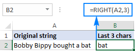
For example, to extract the last 3 characters from the string in cell A2, use this formula:
=RIGHT(A2, 3)
The result might look something similar to this:
Important note! The Excel RIGHT function always returns a text string, even if the original value is a number. To force a Right formula to output a number, use it in combination with the VALUE function as demonstrated in this example.
How to use RIGHT function in Excel - formula examples
In real-life worksheets, the Excel RIGHT function is rarely used on its own. In most cases, you will be using it together with other Excel functions as part of more complex formulas.
How to get a substring that comes after a certain character
In case you want to extract a substring that follows a specific character, use either SEARCH or FIND function to determine the position of that character, subtract the position from the total string length returned by the LEN function, and pull that many characters from the rightmost side of the original string.
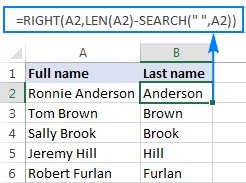
Let's say, cell A2 contains the first and last name separated by a space, and you aim to pull the last name to another cell. Just take the generic formula above and you put A2 in place of string, and " " (space) in pace of character:
=RIGHT(A2,LEN(A2)-SEARCH(" ",A2))
The formula will yield the following result:
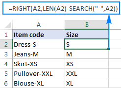
In a similar manner, you can get a substring that follows any other character, e.g. a comma, semicolon, hyphen, etc. For example, to extract a substring that comes after a hyphen, use this formula:
=RIGHT(A2,LEN(A2)-SEARCH("-",A2))
The result will look similar to this:
How to extract a substring after the last occurrence of the delimiter
When dealing with complex strings that contain several occurrences of the same delimiter, you may often need to retrieve the text to the right of the last delimiter occurrence. To make things easier to understand, have a look at the following source data and desired result:

As you can see in the screenshot above, Column A contains a list of errors. Your goal is to pull the error description that comes after the last colon in each string. An additional complication is that the original strings may contain different numbers of delimiter instances, e.g. A3 contains 3 colons while A5 just one.
The key to finding a solution is determine the position of the last delimiter in the source string (the last occurrence of a colon in this example). To do this, you will need to use a handful of different functions:
- Get the number of delimiters in the original string. It's an easy part:
- Firstly, you calculate the total length of the string using the LEN function: LEN(A2)
- Secondly, you compute the length of the string without delimiters by using the SUBSTITUTE function that replaces all occurrences of a colon with nothing: LEN(SUBSTITUTE(A2,":",""))
- Finally, you subtract the length of the original string without delimiters from the total string length: LEN(A2)-LEN(SUBSTITUTE(A2,":",""))
To make sure the formula works right, you can enter it in a separate cell, and the result will be 2, which is the number of colons in cell A2.
- Replace the last delimiter with some unique character. In order to extract the text that comes after the last delimiter in the string, we need to "mark" that final occurrence of the delimiter in some way. For this, let's replace the last occurrence of a colon with a character that does not appear anywhere in the original strings, for example with a pound sign (#).
If you are familiar with the syntax of the Excel SUBSTITUTE function, you may remember that it has the 4th optional argument (instance_num) that allows replacing only a specific occurrence of the specified character. And since we have already calculated the number of delimiters in the string, simply supply the above function in the fourth argument of another SUBSTITUTE function:
=SUBSTITUTE(A2,":","#",LEN(A2)-LEN(SUBSTITUTE(A2,":","")))If you put this formula in a separate cell, it would return this string: ERROR:432#Connection timed out
- Get the position of the last delimiter in the string. Depending on what character you replaced the last delimiter with, use either case-insensitive SEARCH or case-sensitive FIND to determine the position of that character in the string. We replaced the last colon with the # sign, so we use the following formula to find out its position:
=SEARCH("#", SUBSTITUTE(A2,":","#",LEN(A2)-LEN(SUBSTITUTE(A2,":",""))))In this example, the formula returns 10, which is the position of # in the replaced string.
- Return a substring to the right of the last delimiter. Now that you know the position of the last delimiter in a string, all you have to do is subtract that number from the total string length, and get the RIGHT function to return that many characters from the end of the original string:
=RIGHT(A2,LEN(A2)-SEARCH("$",SUBSTITUTE(A2,":","$",LEN(A2)-LEN(SUBSTITUTE(A2,":","")))))
As shown in the screenshot below, the formula works perfectly:

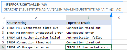
If you are working with a large dataset where different cells may contain different delimiters, you may want to enclose the above formula in the IFERROR function to prevent possible errors:
=IFERROR(RIGHT(A2,LEN(A2)-SEARCH("$",SUBSTITUTE(A2,":","$",LEN(A2)-LEN(SUBSTITUTE(A2,":",""))))), A2)
In case a certain string does not contain a single occurrence of the specified delimiter, the original string will be returned, like in row 6 in the screenshot below:
How to remove the first N characters from a string
Apart from extracting a substring from the end of a string, the Excel RIGHT function comes in handy in situations when you want to remove a certain number of characters from the beginning of the string.
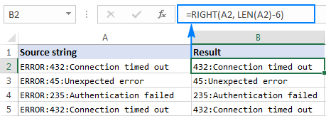
In the dataset used in the previous example, you may want to remove the word "ERROR" that appears at the start of each string and leave only the error number and description. To have it done, subtract the number of characters to be removed from the total string length, and supply that number to the num_chars argument of the Excel RIGHT function:
In this example, we remove the first 6 characters (5 letters and a colon) from the text string in A2, so our formula goes as follows:
=RIGHT(A2, LEN(A2)-6)
Can the Excel RIGHT function return a number?
As mentioned in the beginning of this tutorial, the RIGHT function in Excel always returns a text string even if the original value is a number. But what if you work with a numeric dataset and want the output to be numeric too? An easy workaround is nesting a Right formula in the VALUE function, which is specially designed to convert a string representing a number to a number.
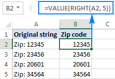
For example, to pull the last 5 characters (zip code) from the string in A2 and convert the extracted characters to a number, use this formula:
=VALUE(RIGHT(A2, 5))
The screenshot below shows the result - please notice the right-aligning numbers in column B, as opposed to left-aligned text strings in column A:
Why doesn't the RIGHT function work with dates?
Since the Excel RIGHT function is designed to work with text strings whereas dates are represented by numbers in the internal Excel system, a Right formula is unable to retrieve an individual part of a date such as a day, month or year. If you attempt to do this, all you will get is a few last digits of the number representing a date.
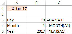
Supposing, you have the date 18-Jan-2017 in cell A1. If you try to extract the year with the formula RIGHT(A1,4), the result would be 2753, which is the last 4 digits of number 42753 that represents January 18, 2017 in the Excel system.

"So, how do I retrieve a certain part of a date?", you may ask me. By using one of the following functions:
- DAY function to extract a day: =DAY(A1)
- MONTH function to get a month: =MONTH(A1)
- YEAR function to pull a year: =YEAR(A1)
The following screenshot shows the results:
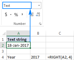
If your dates are represented by text strings, which is often the case when you export data from an external source, nothing prevents you from using the RIGHT function to pull the last few characters in the string that represent a certain part of the date:
Excel RIGHT function not working - reasons and solutions
If a Right formula does not work right in your worksheet, most likely it's because of one of the following reasons:
- There is one or more trailing spaces in the original data. To quickly remove extra spaces in cells, use either the Excel TRIM function or the Trim spaces tool.
- The num_chars argument is less than zero. Of course, you will hardly want to put a negative number in your formula on purpose, but if the num_chars argument is calculated by another Excel function or a combination of different functions and your Right formula returns the #VALUE! error, be sure to check the nested function(s) for errors.
- The original value is a date. If you have followed this tutorial closely, you already know why the RIGHT function cannot work with dates. If someone skipped the previous section, you can find full details in Why the Excel RIGHT function does not work with dates.
This is how you use the RIGHT function in Excel. To have a closer look at the formulas discussed in this tutorial, you are most welcome to download our sample workbook below. I thank you for reading and hope to see you on our blog next week.
Available downloads
Excel RIGHT function - examples (.xlsx file)
 by
by
121 comments
I have a list of dates, and I want to extract just the number after the ":" from a specified date. The date is being specified with a cell reference. For example in the below data (which is all contained in one cell) I want extract the number 20 since the cell reference is 2022:
3/3/2024:21,12/2/2023:22,8/31/2023:19,7/31/2023:19,1/7/2023:22,5/19/2022:20,11/30/2021:17,4/30/2021:18,10/9/2020:18,5/11/2020:17
Hi! Based on your description, it is hard to completely understand your task. However, I’ll try to guess and offer you the following formula:
=MID(A1,SEARCH("2022",A1)+5,2)
For more information, please visit: Excel substring: how to extract text from cell.
Rubiyat-Dhaka-Age31-Blood Group B+
I want to get "Blood Group B+" from above data. Whatever in the last cell before the last "-". Kindly assist.
Hi! You can find the answer to your question in this guide: How to extract last word in Excel.
For example:
=TRIM(RIGHT(SUBSTITUTE(A1, "-", REPT(" ", LEN(A1))), LEN(A1)))
Thank you
Helped a lot. Thanks.
Description Output
IMPS CR ECMS-9229-3357-RAJESH-058905500070 058905500070
IMPS CR ECMS-9002-3357-SURESH-00000037843521283 00000037843521283
IMPS CR ECMS-9026-3357-LOKESH-640701010050314 640701010050314
IMPS CR ECMS-9026-3357-RAVI-640701010050314 640701010050314
IMPS CR ECMS-9026-3357-RAJU-130111100001972 130111100001972
Above description is details. I want Output data. Is there any formula ???
Hi! To extract text after the last occurrence of a specific character, use TEXTAFTER function with parameter [instance_num] -1
=TEXTAFTER(A1,"-",-1)
You can also use this instruction: How to extract last word in Excel.
Try this formula:
=TRIM(RIGHT(SUBSTITUTE(A1, "-", REPT(" ", LEN(A1))), LEN(A1)))
I hope my advice will help you solve your task.
Hi. I need help.
I have a cell with 4 options A,O,LA-**, and EL-**. The latter 2 are followed by time. from that cell I need to fill 4 time stamp cells. For example:
EL-13:00 (stands for leaving at 1PM). I need to have 4 values from that cell. 1. In at 8:00, 2. out at 12:00 3. In at 12:30 4. Early Out at 13:00 for the end of day where normally it would be 16:30. I tried to put a Right, Len formula to remove the 1st 3 characters and use the results in a greater than, less than IF function but my results were not accurate. I ended up with this formula:
Cell 1. IF(ISBLANK($B32),"",IF($B32="O",8/24,IF(($B32="A"),"AB",IF(COUNTIF($B32,"LA*"),RIGHT($B32,LEN($B32)-3),IF(COUNTIF($B32,"EL*"),RIGHT($B32,LEN($B32)-3)))))).
Cell 2. IF(ISBLANK($B32),"",IF($B32="O",12/24,IF(($B32="A"),"AB",IF(COUNTIF($B32,"LA*"),RIGHT($B32,LEN($B32)-3),IF(COUNTIF($B32,"EL*"),RIGHT($B32,LEN($B32)-3)))))).
Cell 3. IF(ISBLANK($B32),"",IF($B32="O",12.5/24,IF(($B32="A"),"AB",IF(COUNTIF($B32,"LA*"),RIGHT($B32,LEN($B32)-3),IF(COUNTIF($B32,"EL*"),RIGHT($B32,LEN($B32)-3)))))).
Cell 4. IF(ISBLANK($B32),"",IF($B32="O",16.5/24,IF(($B32="A"),"AB",IF(COUNTIF($B32,"LA*"),RIGHT($B32,LEN($B32)-3),IF(COUNTIF($B32,"EL*"),RIGHT($B32,LEN($B32)-3)))))).
That formula gives me the same number across the 4 cells for LA-, and EL-. I tried to enter an IF, and formula with right, Len did not work.
a AB AB AB AB
o 8:00 12:00 12:30 16:30
LA-10:07 10:07 10:07 10:07 10:07
EL-14:19 14:19 14:19 14:19 14:19
EL-10:20 10:20 10:20 10:20 10:20
I need it to be:
a AB AB AB AB
o 8:00 12:00 12:30 16:30
LA-10:07 10:07 12:00 12:30 16:30
EL-14:19 8:00 12:00 12:30 14:19
EL-10:20 8:00 10:20
I tried using IF(AND(RIGHT(b32,LEN(b32)-3)>8/24, RIGHT(b32,LEN(b32)-3)<12/24),RIGHT(b32,LEN(b32)-3),"No") within the above formula but the results were not accurate. It seems that the Right and len does not work within the IF, and formula.
I would extremely appreciate your point of view. I have been working on this for a few days now but nothing is working.
Thanks
Hi! If I understand the problem correctly, the text function RIGHT returns text, not time. Try converting the text to a number and change the formula:
=IF(ISBLANK($B32),"",IF($B32="O",8/24,IF(($B32="A"),"AB",IF(COUNTIF($B32,"LA*"),--RIGHT($B32,LEN($B32)-3),IF(COUNTIF($B32,"EL*"),--RIGHT($B32,LEN($B32)-3))))))
Hope this is what you need.
I need to extract the 5 digit code 263855 within the string:
/ABCVX/Files/PROJECTS/FILES/DTPA (ABCDEFGH)
(263855)/STAT/POOLING/ANALYSIS_99/METADATA
I tried: =RIGHT(B2,LEN(B58)-SEARCH("$",SUBSTITUTE(B2,"(","$",LEN(B2)-LEN(SUBSTITUTE(B2,"(","")))))
But how do I just extract the following 5 digits, and not the entore rest of the string?
For your text string, you can use substring functions:
=MID(B2,SEARCH("#",SUBSTITUTE(B2,"(","#",2))+1,6)
Please check out this article to learn how to extract substring that match a pattern: Regex to extract strings in Excel (one or all matches). Use this formula:
=RegExpExtract(B2, "\d{6}", 1)
I recommend paying attention to the Regex tool. You can find, extract, compare, delete, or replace strings that match the regular expression pattern you enter. You don't need to install any VBA code. The tool is included in the Ultimate Suite for Excel and can be used in a free trial to see how it works.
{ "STATE": "Alabama", "CODE": "AL"} i want to extract the text "AL", how to do it.??
I believe the following formula will help you solve your task:
=CHOOSECOLS(TEXTSPLIT(A1,""""),8)
To split text into parts using delimiters, use the TEXTSPLIT function. To select a specific part of the text, use the CHOOSECOLS function.
The number of characters I want to grab from a table changes.
Meaning sometimes I want to grab the right 9 characters, and sometimes I want to grab the right 15 characters. Is there a way to achieve this with one formula so I can drag down, rather than adjusting them all?
Hi! Use a cell reference in the formula that will write the number of characters 9 or 15.
I have this: T1234LA. But i want it to be T-1234LA.
How do I achieve that using right function so it can affect the other column(drop down)
Hi! To insert a character at a specific position in a text string, you can use the REPLACE function.
=REPLACE(A4,2,0,"-")
Hi If the text extracted from the cell is a number, can i use this in for a seperate equation?
Ex.
A1 = 45, 6
A2 = 53, 3
I can extract the numbers to the right or left of the comma into another cell. However when I try to eg. sum all the numbers on the right of the comma it returns as 0. Is it possible?
Thanks in advance!
Hello! When you extract a number to the right of a comma, it is returned as text. Convert this text to a number, such as this:
=--TEXTAFTER(A1,",")
For more information, please visit: How to convert text to number in Excel.
How can I test the last digit of a SUM(range) result see if it is zero eg SUM(A4:A8) = 1234.70.
The RIGHT function always returns '7'.
Hello! The last digit of your number is 7. You see 0 because the number format is set to two decimal places. The real number is 1234.7.
If you use the TEXT function to convert the number to text in the desired format, the last digit can be 0.
TEXT(SUM(A4:A8), "#.00") will return the text "1234.70"
I have a data like Shaym M Sunny, Suraj T S, them how can I extract the last name eg: Sunny and S from the names)
Hi! Here is the article that may be helpful to you: How to separate names in Excel: split first and last name into different columns.
Hi! I need your help.
I'm trying to use the RIGHT formula for this:
For instance:
A1: 24.0
I need "0" only to B1 cell.
Please help! thank you!
Please re-check the article above since it covers your task.
I want to remove last alphabets only character please suggest complete excel formula
LC21I142A
LC21L090L
LC21L093A
LC21L053C
Count the number of characters with the LEN function and extract all except the last character with the LEFT function. You can also delete the last character with the REPLACE function.
You can use these formulas:
=LEFT(A2,LEN(A2)-1)
=REPLACE(A2,LEN(A2),1,"")
Hello , i have some problem with this
i want to get this text as different coloumns
may can help me
Example : Name / Full name 123456789
how do i get the name , full name , and the number in different coloumns , thankyou .
Hi!
You can find the examples and detailed instructions here: Split string by delimiter or pattern, separate text and numbers. You can also use the new TEXTSPLIT function to split the text into cells.
Hi thanks for the clear explanation! I am trying to use the LEFT and RIGHT functions in conjunction with each other that concatenates the number of characters specified in Data Cell 02 from the left and right ends of the content in Data Cell 01.
data cell 1:
12abcd12
data cell 2:
2
Hi!
If I understand your task correctly, try the following formula:
=LEFT(A1,A2)&RIGHT(A1,A2)
For more information, please read: Combine text strings, cells and columns.
hi i please help me get the right formula:
ex.25,00
=RIGHT(A1;2)
i used the following formula: =RIGHT(A1,2) and the result was 25
?????
Thank you so much!
Hi!
If a number is written in A1, then this is 25. You use the "Number" format in the cell. You can convert number to text using the TEXT function in the format you need.
For example -
=TEXT(A2, "0.00")
Is there a way to use conditional If...then statements within a Right formula? For instance, I have a series of numbers that I would like to sort by the last number, not necessarily the last digit, because some numbers have a letter (or two) at the end, ie 1234A, 43353CC, 67890, etc. So they should be sorted in descending order according to 4, 3, and 0, but because the position of the last number changes, can't use a simple formula. How would I do this?
Hello!
To extract the last digit from text, you can use the RIGHT function and these guidelines: How to extract number from the end of text string.
=RIGHT(RIGHT(A2, LEN(A2) - MAX(IF(ISNUMBER(MID(A2, ROW(INDIRECT("1:"&LEN(A2))), 1) *1)=FALSE, ROW(INDIRECT("1:"&LEN(A2))), 0))),1)