In the last few articles, we've discussed different Text functions - those that are used to manipulate text strings. Today our focus is on the RIGHT function, which is designed to return a specified number of characters from the rightmost side of a string. Like other Excel Text functions, RIGHT is very simple and straightforward, nevertheless it has a few unobvious uses that might prove helpful in your work.
Excel RIGHT function syntax
The RIGHT function in Excel returns the specified number of characters from the end of a text string.
The syntax of the RIGHT function is as follows:
Where:
- Text (required) - the text string from which you want to extract characters.
- Num_chars (optional) - the number of characters to extract, starting from the rightmost character.
- If num_chars is omitted, 1 last character of the string is returned (default).
- If num_chars is greater than the total number of characters in the string, all characters are returned.
- If num_chars is a negative number, a Right formula returns the #VALUE! error.
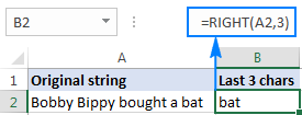
For example, to extract the last 3 characters from the string in cell A2, use this formula:
=RIGHT(A2, 3)
The result might look something similar to this:
Important note! The Excel RIGHT function always returns a text string, even if the original value is a number. To force a Right formula to output a number, use it in combination with the VALUE function as demonstrated in this example.
How to use RIGHT function in Excel - formula examples
In real-life worksheets, the Excel RIGHT function is rarely used on its own. In most cases, you will be using it together with other Excel functions as part of more complex formulas.
How to get a substring that comes after a certain character
In case you want to extract a substring that follows a specific character, use either SEARCH or FIND function to determine the position of that character, subtract the position from the total string length returned by the LEN function, and pull that many characters from the rightmost side of the original string.
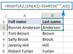
Let's say, cell A2 contains the first and last name separated by a space, and you aim to pull the last name to another cell. Just take the generic formula above and you put A2 in place of string, and " " (space) in pace of character:
=RIGHT(A2,LEN(A2)-SEARCH(" ",A2))
The formula will yield the following result:
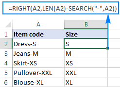
In a similar manner, you can get a substring that follows any other character, e.g. a comma, semicolon, hyphen, etc. For example, to extract a substring that comes after a hyphen, use this formula:
=RIGHT(A2,LEN(A2)-SEARCH("-",A2))
The result will look similar to this:
How to extract a substring after the last occurrence of the delimiter
When dealing with complex strings that contain several occurrences of the same delimiter, you may often need to retrieve the text to the right of the last delimiter occurrence. To make things easier to understand, have a look at the following source data and desired result:

As you can see in the screenshot above, Column A contains a list of errors. Your goal is to pull the error description that comes after the last colon in each string. An additional complication is that the original strings may contain different numbers of delimiter instances, e.g. A3 contains 3 colons while A5 just one.
The key to finding a solution is determine the position of the last delimiter in the source string (the last occurrence of a colon in this example). To do this, you will need to use a handful of different functions:
- Get the number of delimiters in the original string. It's an easy part:
- Firstly, you calculate the total length of the string using the LEN function: LEN(A2)
- Secondly, you compute the length of the string without delimiters by using the SUBSTITUTE function that replaces all occurrences of a colon with nothing: LEN(SUBSTITUTE(A2,":",""))
- Finally, you subtract the length of the original string without delimiters from the total string length: LEN(A2)-LEN(SUBSTITUTE(A2,":",""))
To make sure the formula works right, you can enter it in a separate cell, and the result will be 2, which is the number of colons in cell A2.
- Replace the last delimiter with some unique character. In order to extract the text that comes after the last delimiter in the string, we need to "mark" that final occurrence of the delimiter in some way. For this, let's replace the last occurrence of a colon with a character that does not appear anywhere in the original strings, for example with a pound sign (#).
If you are familiar with the syntax of the Excel SUBSTITUTE function, you may remember that it has the 4th optional argument (instance_num) that allows replacing only a specific occurrence of the specified character. And since we have already calculated the number of delimiters in the string, simply supply the above function in the fourth argument of another SUBSTITUTE function:
=SUBSTITUTE(A2,":","#",LEN(A2)-LEN(SUBSTITUTE(A2,":","")))If you put this formula in a separate cell, it would return this string: ERROR:432#Connection timed out
- Get the position of the last delimiter in the string. Depending on what character you replaced the last delimiter with, use either case-insensitive SEARCH or case-sensitive FIND to determine the position of that character in the string. We replaced the last colon with the # sign, so we use the following formula to find out its position:
=SEARCH("#", SUBSTITUTE(A2,":","#",LEN(A2)-LEN(SUBSTITUTE(A2,":",""))))In this example, the formula returns 10, which is the position of # in the replaced string.
- Return a substring to the right of the last delimiter. Now that you know the position of the last delimiter in a string, all you have to do is subtract that number from the total string length, and get the RIGHT function to return that many characters from the end of the original string:
=RIGHT(A2,LEN(A2)-SEARCH("$",SUBSTITUTE(A2,":","$",LEN(A2)-LEN(SUBSTITUTE(A2,":","")))))
As shown in the screenshot below, the formula works perfectly:

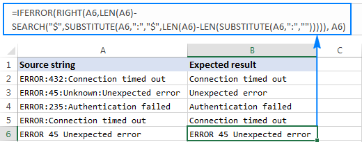
If you are working with a large dataset where different cells may contain different delimiters, you may want to enclose the above formula in the IFERROR function to prevent possible errors:
=IFERROR(RIGHT(A2,LEN(A2)-SEARCH("$",SUBSTITUTE(A2,":","$",LEN(A2)-LEN(SUBSTITUTE(A2,":",""))))), A2)
In case a certain string does not contain a single occurrence of the specified delimiter, the original string will be returned, like in row 6 in the screenshot below:
How to remove the first N characters from a string
Apart from extracting a substring from the end of a string, the Excel RIGHT function comes in handy in situations when you want to remove a certain number of characters from the beginning of the string.
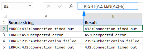
In the dataset used in the previous example, you may want to remove the word "ERROR" that appears at the start of each string and leave only the error number and description. To have it done, subtract the number of characters to be removed from the total string length, and supply that number to the num_chars argument of the Excel RIGHT function:
In this example, we remove the first 6 characters (5 letters and a colon) from the text string in A2, so our formula goes as follows:
=RIGHT(A2, LEN(A2)-6)
Can the Excel RIGHT function return a number?
As mentioned in the beginning of this tutorial, the RIGHT function in Excel always returns a text string even if the original value is a number. But what if you work with a numeric dataset and want the output to be numeric too? An easy workaround is nesting a Right formula in the VALUE function, which is specially designed to convert a string representing a number to a number.
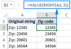
For example, to pull the last 5 characters (zip code) from the string in A2 and convert the extracted characters to a number, use this formula:
=VALUE(RIGHT(A2, 5))
The screenshot below shows the result - please notice the right-aligning numbers in column B, as opposed to left-aligned text strings in column A:
Why doesn't the RIGHT function work with dates?
Since the Excel RIGHT function is designed to work with text strings whereas dates are represented by numbers in the internal Excel system, a Right formula is unable to retrieve an individual part of a date such as a day, month or year. If you attempt to do this, all you will get is a few last digits of the number representing a date.
Supposing, you have the date 18-Jan-2017 in cell A1. If you try to extract the year with the formula RIGHT(A1,4), the result would be 2753, which is the last 4 digits of number 42753 that represents January 18, 2017 in the Excel system.

"So, how do I retrieve a certain part of a date?", you may ask me. By using one of the following functions:
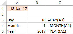
- DAY function to extract a day: =DAY(A1)
- MONTH function to get a month: =MONTH(A1)
- YEAR function to pull a year: =YEAR(A1)
The following screenshot shows the results:
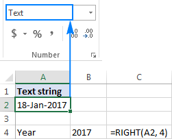
If your dates are represented by text strings, which is often the case when you export data from an external source, nothing prevents you from using the RIGHT function to pull the last few characters in the string that represent a certain part of the date:
Excel RIGHT function not working - reasons and solutions
If a Right formula does not work right in your worksheet, most likely it's because of one of the following reasons:
- There is one or more trailing spaces in the original data. To quickly remove extra spaces in cells, use either the Excel TRIM function or the Trim spaces tool.
- The num_chars argument is less than zero. Of course, you will hardly want to put a negative number in your formula on purpose, but if the num_chars argument is calculated by another Excel function or a combination of different functions and your Right formula returns the #VALUE! error, be sure to check the nested function(s) for errors.
- The original value is a date. If you have followed this tutorial closely, you already know why the RIGHT function cannot work with dates. If someone skipped the previous section, you can find full details in Why the Excel RIGHT function does not work with dates.
This is how you use the RIGHT function in Excel. To have a closer look at the formulas discussed in this tutorial, you are most welcome to download our sample workbook below. I thank you for reading and hope to see you on our blog next week.
Available downloads
Excel RIGHT function - examples (.xlsx file)
 by
by
128 comments
I have a sentence mail.google.com, mail.yahoo.com... in column
I want to replace with mail_google.com, etc.
Hi!
To find and replace text in a cell, use the SUBSTITUTE function:
=SUBSTITUTE(A1,"mail.","mail_")
This should solve your task.
If I have common.annualRevenu.test, bdf.annualRevenu.test
to -- > common_annualRevenu.test, bdf_annualRevenu.test
then how it works?
Please.
Hello!
To replace characters in text, use SUBSTITUTE function.
=SUBSTITUTE(SUBSTITUTE(A1,".","_",3),".","_",1)
Hope this is what you need.
I could use some help please. How can I extract all characters to the right of the last pipe and space even when some strings have 1 or multiple pipes?
Example 1: Automotive/RV | Compasses - Magnetic,Marine Navigation & Instruments | Compasses,Marine Navigation & Instruments | Safety
Result 1: Safety
Example 2: Marine Navigation & Instruments | Safety
Result 2: Safety
I figured it out from the download example:
=RIGHT(E16,LEN(E16)-FIND("$",SUBSTITUTE(E16,"|","$",LEN(E16)-LEN(SUBSTITUTE(E16,"|",""))))-1)
Hello!
If I got you right, the formula below will help you with your task:
=RIGHT(A1,LEN(A1)-SEARCH("#",SUBSTITUTE(A1,"|","#",LEN(A1) - LEN(SUBSTITUTE(A1,"|",""))))-1)
Hi there!
thanks a bunch for your help.
I have this text on A1:
10.1.4.81'
I have this text on A2:
10.1.20.234
In need to figure out the position of the first "." starting from the RIGHT.
So I am expecting the results:
3
4
I cannot make it :(
Much appreciated,
Josu.
Hello!
Replace the last "." to "#" using the SUBSTITUTE function.
The formula below will do the trick for you:
=LEN(A1)-SEARCH("#",SUBSTITUTE(A1,".","#",LEN(A1) - LEN(SUBSTITUTE(A1,".",""))))+1
This should solve your task.
I need a formula that can convert text in the format 2/15/2022 2:16:09 PM to date and time dd-mmm-yyyy hh:mm [gives 15-Jan-2022 14:16] and should be able to work correctly even where the date provided is 12/31/2022 2:16:09 PM still in the same format [should give 31-Dec-2022 14:16]
Hello!
Try this formula:
=DATE(MID(A2,SEARCH("/",A2,SEARCH("/",A2)+1)+1,4), LEFT(A2, SEARCH("/",A2,1)-1), (MID(A2,SEARCH("/",A2)+1, SEARCH("/",A2,SEARCH("/",A2)+1)- SEARCH("/",A2)-1)))+ MID(A2,SEARCH(" ",A2)+1,20)
We have a ready-made solution for your task. I'd recommend you to have a look at our Text To Date Tool. It parses over 500 combinations representing dates in text format and converts them to regular Excel dates.
HI,
do you know of a good way to extract a word or phrase from a cell containing many words? i'm trying to extract "ticker" or "hero" or "hero 2" or "sidekick" using a formula so we know the location of the message. i tried doing a search function but i could only go two deep due to the errors.
=IFERROR(IF(SEARCH("sidekick",A1)>0,"sidekick","no"),IF(SEARCH("hero",A1)>0,"hero","no"))
header|click|ticker Take 10% off orders $129+ -- i'm trying to extract just "ticker"
homepage|click|hero C2002-ECOM @ $99 -- i'm trying to extract just "hero"
homepage|click|hero 2 Disaster Prep -- i'm trying to extract just "hero 2"
homepage|click|sidekick The BEST Deals This Month -- i'm trying to extract just "sidekick"
Hello!
Using the formula, you can extract the first word after the last separator "|" :
=LEFT(MID(SUBSTITUTE(A1,"|","#", LEN(A1)-LEN(SUBSTITUTE(A1,"|",""))), SEARCH("#",SUBSTITUTE(A1,"|","#",LEN(A1)-LEN(SUBSTITUTE(A1,"|",""))))+1,100), SEARCH(" ",MID(SUBSTITUTE(A1,"|","#",LEN(A1)-LEN(SUBSTITUTE(A1,"|",""))), SEARCH("#",SUBSTITUTE(A1,"|","#",LEN(A1)-LEN(SUBSTITUTE(A1,"|",""))))+1,100))-1)
I have a cell that includes the following (as an example) #14 Wisconsin at #3 Illinois.
I want to extract the state names into different cells. Is successfully isolated "Wisconsin" into a cell using your page on MID and SEARCH ("=MID(A3, SEARCH(" ",A3)+1, SEARCH(" ",A3, SEARCH(" ", A3)+1)-SEARCH(" ",A3)-1)" .
I am struggling to isolate "Illinois". I was trying to use the RIGHT LEN AND FIND functions in combination to no avail.
Any suggestion
Hi!
To extract the last word from the text, use the formula:
=RIGHT(SUBSTITUTE(A3," ","@",LEN(A3)-LEN(SUBSTITUTE(A3," ",""))), LEN(A3)-FIND("@",SUBSTITUTE(A3," ","@",LEN(A3) - LEN(SUBSTITUTE(A3," ",""))),1))
I hope my advice will help you solve your task.
I thought for a moment it worked, but I failed to anticipate something that complicates this.
In some cases what I am extracting is two words. For example #11 Texas at #42 Oklahoma St resulted in just "St" when I want " Oklahoma St" and for #7 Kansas at #19 W Virginia it resulted in just "W" when I need "W Virgnia"
This solution results in only the St being extracted from Oklahoma St - is there a way to tell excel that I need everything after the last space before the name.
Another suggestion is appreciated. It is so close.
Hi!
I wrote this formula based on the description you provided in your original comment. If you gave the correct description of the problem, time would not be wasted.
Try the following formula:
=MID(A1,SEARCH(" ",A1,SEARCH("#",A1,LEN(A1)-LEN(SUBSTITUTE(A1,"#",""))))+1,50)
Hi All,
I need to remove the first two digits from my excel cells if the length of the characters in greater than 10, i.e. I have cell phone numbers and the I want to remove the country code 91 from the cell phone numbers. I know the RIGHT Formula in excel =RIGHT(A1, LEN(A1)-2). But I need to use it with IF condition. I am trying this but it is not working. Can someone please help: =IF(LEN(A1>10) RIGHT (A1, LEN(A1)-2))
Hi!
Please check the formula below, it should work for you:
=IF(LEN(A1)>10,RIGHT(A1,LEN(A1)-2),A1)
Almost there for me, i just need help please, im trying to get the 6 characters that appear after the second to last backslash.
eg. in
\orange rule\apples are nice\pears rock\berrys are yum\strawberry
i need to get 'berrys' (its always 6 characters and always starts after the second to last backslash)
Hello!
Please use the following formula:
=MID(A2,SEARCH("#",SUBSTITUTE(A2,"\","#",LEN(A2)-LEN(SUBSTITUTE(A2,"\",""))-1))+1,6)
This should solve your task.
Hi Please help me with the below questions answer.
Input:
cast(trim(name) as string) as name
Null as address
Cast(id as decimal(38,10)) as id
Output:
Name
Address
Id
Hi!
To extract a string from the middle of the text, use the MID function.
Hi,
I have the following descriptions in my excel file.
"And[wondering looked a] me.
Her h[ir was thick ]ith many a curl
She w[s eight years old she s]id;
How ma[y may you b]?"
I need to extract the last word after the string "]". Can you please help with the formula?
By the way, I used CONCATENATE(A1,",",A2,"," so on and so forth. However, if cells are empty it displays a comma.
Something like this
125306920, 125298912,125297627,,,,,,,,,,
Hi Everyone,
Good day to all! I don't know what to use or how to use the code. But what I need is put a comma after every 9th number.
Column A
125306920
125298912
125297627
125300893
125311521
125306307
And if i use CONCATENATE i get this result 125306920125298912125297627125300893125311521125306307. Please help.
Thanks a lot!
Hello!
To combine delimited text, use the TEXTJOIN function. Read more in this guide.
I hope I answered your question.
Good day! TEXTJOIN doesn't seem to work in 2013, if it's a plugin/addin i'm not allowed to download it either. :(
Hi,
Unfortunately, in Excel2013 you can use either the CONCATENATE function or the VBA macro.
Hello guys,
Can you help me with this. I want to achieve the column B result given the column A as my data.
In column A: ThePLAN 599 With iPhone 12 128GB Red
ThePLAN 2799 with iPhone 12 Pro Max 256GB Gold
ThePLAN PLUS 2999 (Consumable 1299)
ThePLAN PLUS 599 (Consumable 299)
Column B shows:
iPhone 12 128GB Red
iPhone 12 Pro Max 256GB Gold
TPP
TPP
Thank you,
Hello!
If I understand your task correctly, the following formula should work for you:
=IFERROR(RIGHT(A1,LEN(A1)-SEARCH("with",A1,1)-4),"TPP")
I hope it’ll be helpful.
Woah! it really worked! Thanks a lot!!!!
HOW CAN WE GET NUMBER AFTER THE LAST COMMA IN EXCEL
question - 1, 2, 5, 25, 223
answer should be 223
question - 1,2,5,25, 42
answer should be 42
Hello!
The formula below will do the trick for you:
=RIGHT(SUBSTITUTE(C1,",","#", LEN(C1)-LEN(SUBSTITUTE(C1,",",""))), LEN(C1)-FIND("#",SUBSTITUTE(C1,",","#", LEN(C1)-LEN(SUBSTITUTE(C1,",",""))),1))
Hope this is what you need.
Hi. what function (and how) do I have to use with this given data?
ECON:F6797-1111
ECON:M9350-1
CS:F5738-1111
AC:M4799-1111
HRDM:M7415-111
AC:M7056-1111
1 = 2016-2017
11 = 2017-2018
111 = 2018-2019
1111 = 2019-2020
only the last character. I know how to extract the (1,11,111,111 with this function =RIGHT(A2,LEN(A2)-SEARCH("-",A2))) but I do not know how to replace those values according to its year equivalent.
I need to substitute the rightmost character so that my column will sort properly:
if rightmost ="a", make it ".1"
if rightmost ="b", make it ".2"
I've tried everything but I don't get the result I need. Please help.
Hello
Here is the formula that should work perfectly for you:
=IF(RIGHT(C1,1)="a",REPLACE(C1,LEN(C1),1,".1"), IF(RIGHT(C1,1)="b",REPLACE(C1,LEN(C1),1,".2")))
Hope this is what you need.
Team, I hope this message finds you and your families all doing well. Need help and can't seem to get Excel to do what I want. I have an excel spreadsheet with IP addresses e.g. 10.9.1.100 I want to subtract the last Octet by 1 and have the output return the revised IP address.
Example: Column A2 10.9.1.100
Column A3 (suggested Formula)
Column A4 output from A3 10.9.1.99
Thank you for any help you can provide
Hello!
If I understand your task correctly, the following formula should work for you:
=LEFT(A2,SEARCH("#",SUBSTITUTE(A2,".","#",3),1)) & (--MID(A2,SEARCH("#",SUBSTITUTE(A2,".","#",3),1)+1, LEN(A2)-SEARCH("#",SUBSTITUTE(A2,".","#",3),1))-1)
I hope this will help
Hi Team,
How can i extract the file name alone in the below mentioned link, like "Input form.xlsb" cause the file name will dynamic one.can you help me
C:\Users\UST901\Desktop\Confidential\New Report\Input form.xlsb
Thanks\Raju
Hello!
I have a text in a cell. Sometimes this text has at the end one empty space (it is visible only if I enter in the cell and go with the cursor to the most right of the text in the cell). I would like to use the right function (or any other function if feasible) in order to take this empty space out of the text in the cell (however the tricky part is that the formula should work only if there is a space in the end of the text, if it is a symbol it should not change the text. Also the formula should not delete other empty spaces within the text, only the empty space at the end of the text). Thanks!
Hello Ivan!
If I understand your task correctly, the following formula should work for you:
=IF(RIGHT(D1,1)=" ",REPLACE(D1,LEN(D1),1,""),D1)
I hope this will help
Hi, I too needed the below case? out put last 4 digit from the different lenth of datas as below.
Original: To be
ABCDEF-12345 ABCD-2345
ABCD-23456 ABCD-3456
ABC-34567 ABC-4567
AB-45678 AB-5678
Thanks in advance.
Hello!
I hope you have studied the recommendations in the above tutorial. To display the last 4 digits as number, use the RIGHT function, as described in the article above
=--RIGHT(A1,4)
I want to exclude the last 2 caracters
Please see the following string:
Cell A1 = Arch Psychological Services 39-9912 106 Street, Edmonton, Alberta T5K 1C5
I am trying to separate the name of the business and the address as follows:
Cell B1 = Arch Psychological Services
Cell C1 = 39-9912 106 Street, Edmonton, Alberta T5K 1C5
How would you use the RIGHT function? or any other function?
Thanks
Hello ,
I want the output this type 101, 1000, 102.
Please Give me a solution.
1. ZSW234ER101
2. ZSW234ER1000
3. ZSW234ER102
Hello! You can use regular expressions and the user-defined function RegExpExtract to extract numbers from text by pattern. You can find the examples and detailed instructions here: How to extract substrings in Excel using regular expressions (Regex).
The formula below will do the trick for you:
=RegExpExtract(A1, "(\d+)(?!.*\d)")
I recommend paying attention to the Regex tool. You can find, extract, compare, delete, or replace strings that match the regular expression pattern you enter.
Help Please, this is eating my brain.
I have a Title String example
ex: Title = Waterfront (0000000) created 11/18/2019 8:47 AM | Kitchen | Morgan Stanley | Georgia | Ashok Masetty
I need value "Georgia" and "Ashok Masetty" seperately but I am getting "Georgia | Ashok Masetty" using the below formula
=RIGHT(RIGHT(RIGHT(Title,LEN(Title)-INT(FIND("|",Title))),LEN(RIGHT(Title,LEN(Title)-INT(FIND("|",Title))))-INT(FIND("|",RIGHT(Title,LEN(Title)-INT(FIND("|",Title)))))),LEN(RIGHT(RIGHT(Title,LEN(Title)-INT(FIND("|",Title))),LEN(RIGHT(Title,LEN(Title)-INT(FIND("|",Title))))-INT(FIND("|",RIGHT(Title,LEN(Title)-INT(FIND("|",Title)))))))-INT(FIND("|",RIGHT(RIGHT(Title,LEN(Title)-INT(FIND("|",Title))),LEN(RIGHT(Title,LEN(Title)-INT(FIND("|",Title))))-INT(FIND("|",RIGHT(Title,LEN(Title)-INT(FIND("|",Title)))))))))
Any help is appreciated.
Thanks
I have set of alphanumeric employee ID, like 00PTPL-001 next will be 00PTLP-00101, length of alphanumeric ID is not same of all. From this ID I need to extract ID by removing first two zeroes and last two digits if added with employee ID. Unable to use MID function, because both sides of colon text has to be extracted. Kindly help with one dynamic formula to remove leading and trailing unwanted digits and texts.
Hi,
this formula did not work for me. the formula brought the same text back. no change. any idea why?
Lidia
Hi,
I'm using Right and Left functions to get the first and last names on a cell, they are separated by comma. The solution doesn't bring up the total number of values before and after the comma i.e. for the full name "Soberado,Veronica"
The Left function (without -1 at the end) comes as "Soberad" and if I place the "-1" to get the position just before the comma, then it comes as "Sobera".
The Right function comes as "eronica" (missing the V).
This is all part of a bigger equation where I am doing a lookup to find the Full Name in the array and then I separate the name in First and Surname, so not sure if these equations are able to work together or not. See below:
=RIGHT(INDEX(Mob_Database,MATCH($F$15,Mob_Database[Staff_No],0),6),SEARCH(",",Mob_Database[Title]))
I'm a beginner using Excel, so would really appreciate some advice and provide some potential explanation of why this is not working.
Many thanks in advance.
Clara
Hi, if anyone could help with the below case?
Original: To be
ABCDEF-12345 ABCD-2345
ABCD-23456 ABCD-3456
ABC-34567 ABC-4567
AB-45678 AB-5678
Thanks in advance.
David
Hi, anyone could help with the below example ?
Example:
psky90000-11+L1234567.1+Q10000+000000
pshd2b831mm111a+L1234567.11+Q10000+0000”0
How I use the right function formula can get with the L no I need in one column I can fill in 2 type of different data.
Hi if someone could help,
If I have several domains but I get duplicate but different tld (.com, .net, .org, .fr, etc)
what formula can I use to get the tld only ?
Hi Loris,
Is my understanding correct that you want to get only .com, .net, .org, .fr, etc. ? If so, you can use the following formula to extract everything that comes after a dot, including a dot itself:
=IFERROR(RIGHT(A2,LEN(A2)-SEARCH(".",A2)+1), "")
Where A2 is the cell containing the original domain.
I'm using the right and left formula, to separate a number with a coma into to numbers, example:
CELL D18 = 10.50
left cell formula - =LEFT(D18,2) = 10,
the right cell formula =RIGHT(D18,2) = .5
How can I tell the formula to count "0" as part of the number? Taking into account that not all the number's in cell D18 have "0"'s (ex: my D18 cell can be 10.85, in this case the right formula works perfectly).
Thank you,
Carolina
How do I extract the last 2 digits from a date and also add two digits to make an actual date? For example, I was given 925085/15, I need to extract the 15 and include 20 in front of the 15.
I used this formula =RIGHT(A4,2)&"20" and I got 1520 instead of 2015?
Your assistance is appreciated.
hello,
I need your help. I want to extract the numbers inside the brackets from the following:
Access Point 300mb TP-Link WA855RE Range Extender [310575] × 1
Any ideas? I cant figure out the right formula.
Thanks
Hello, Olina,
Thank you for contacting us.
If we understand your task correctly, the formula below should work for you:
=IFERROR(LEFT(RIGHT(A1, LEN(A1)- SEARCH("[",A1) - LEN("[") + 1),SEARCH("]", RIGHT(A1, LEN(A1)- SEARCH("[",A1) - LEN("[") + 1))-1), "")
Alternatively, you can use our Extract Text tool to derive the necessary part of your cell in a few clicks.
Hilyn:
Is the data in Text format or Number format?
If it is in Text try this: =MID(A1,5,2)
This will return the last two characters as text. If it is formatted as a number and needs to be returned as a number then first format it as text and try:
=ABS(MID(A1,5,2)) or =ABS(RIGHT(A1,2))
I can't figure out how to return the last two digits of the number with the trailing zero.
hi i please help me get the right formula:
ex. A1=958.30
i want to copy only the 2 decimal digits which is 30
i used the following formula: =RIGHT(A1,2) and the result was .3
how do i include the "0" ?
Thank you so much!
FORMAT BOTH COLUMNS AS A NUMBER WITH 2 DECIMAL PLACES
HI
I WANT FORMULA AS PER BELOW CONDITION
I/P
MM NO PRICE YEAR VENDOR
O/P
MM NO PRICE LOWEST PRICE IN PARTICULAR YEAR VENDOR
also some records look like this: (comma after state)
XXXX Via Marina, #JXXX, Marina Del Rey, CA, 90292 USA
Gary:
Because I can't see any pattern to the structure of your data, it seems you'll have to handle some of the separation process "By Hand". In other words I don't see any option but for you to clean this data up.
Highlight the cell that contains the data.
Then from the Data tab select Text-to-Columns.
Then click the Delimited button then next.
Then click the Spaces button then next.
Then General then Finish.
Now your data is in separate cells. Problem will be the same type of info is not in the same columns.
You'll have to move the same types into the columns by hand.
If you need to put the name state and zip into one cell you'll need to concatenate them into one cell.
Hi Guys
Need help!
I have an excel file with Addresses that look like this:
"123 Westlawn Unit 134 Los Angles, CA 90066 USA"
"567 Homecoming Dr. #1267 Chino, CA 91708 USA"
I need to Pull City, State and Zip or at least State and Zip. I do not need USA part.
Thank you In advance
Gary
Hi Guys,
I am unable to find the solution for following query, please help me finding the solution.
I want to generate a formula for saving a number to a particular bit column, my table has 9 columns 1,2,3,4,5,6,7,8,9,0 if user input value 20 it should be save in bit 2 column, if user enter value 75 in cell it should be save to column no 7. So guys please suggest me solution and yes i am totally newbie to excel so please give me exact formula to do so.
Thanks in advance.
Thanks for your response Doug
I am using the substitute formula as part of my csv editing arsenal and part of your suggestion to complete the csv :)
But i didn't explain myself correctly i dont think... so in fear of miscommunicating my issue again here is an example.
(Side note) The final csv file must have a heading in cell A1 and all the rows must conform to the standard of the first line: Cell A1 looks like this: lot_number,title,description
This is an example of 1 line of text as it is when i get it: 001,1,2013 CK61FXGP NISSAN MICRA 1.2 VISIA+ AUDIO 5-DR (GREY)(132223 kms)
This is what it needs to look like for the csv end result:
1,2013 CK16XFGP NISSAN MICRA 1.2 VISIA+ AUDIO 5-DR ,(GREY) (132223 kms)
90% of the lines have an open bracket which is the start of the description so i use find and replace to find the first ( and replace it with ,( which is simple enough to get my second comma.
However some lines don't have a description i.e. no open bracket, this is an example of what they would look like: 001,1,2013 CK16XFGP NISSAN MICRA 1.2 VISIA+ AUDIO 5-DR
The part im not getting right is to find all the rows (the list is growing... now up to 400 rows per csv) that don't have the open bracket and add a comma at the end of those lines.
But i'm not sure how to find cells that don't have 2 commas and add a comma to those that only have 1.
Maybe im not looking at it right... hopefully i have explained nicely this time :)
There may be other methods, but this is how I would do it.
I would start by taking the comma off the end of the data so that the data would have the same structure.
Then apply one procedure to all the data.
To get to that point you just need to do some adding and subtracting in a helper column’s cell. Like this:
First, in an open cell, for example, in cell B1, enter =SUBSTITUTE(A1, ",", "", 2)
This should remove the second occurrence of the comma and leave the other comma in place.
Copy this formula down the list to the end of the data.
Now, all the cells have the same structure with one comma in the data, none at the end.
Second, in a new column say cell “C1”, enter =B1&","
This enters a comma at the end of the text from B1.
Then copy down this formula to the end of the data.
When you finish, there is one comma in the data and one comma at the end of the data in column C.
Lastly, you may want to copy the completed data into a new sheet.
If so, copy the data, then in another sheet use “Paste Special – Values”.
This will copy all your data with just one comma in the data and one comma at the end ready for a CSV.
Hi Ablebits team
I work with excel sheets with up to 300 lines of different text in 1 column and need to create a comma delimited csv file which requires a minimum of 2 commas in each line.
Some lines don't have the 2nd comma at the end of the text, how do i go about adding a comma in the cells that are missing the 2nd comma?
Essentially i just need to fine all the cells that are missing a comma at the end of the text and add it in but i haven't a clue how.
Regards Deane
5 Approved 0 Declined & 21 times
6 Approved 3 Declined & 4 times
10 Approved 1 Declined & 14 times
156 Approved 6 Declined & 116 times
always the data comes in the above formate; I want to use conditional formatting in case the first digit > the last digit.
If A:A=2017 then Count K:K
Hi, I have a form in excel which shows a value in a cell of 806.73 (example in field A1).
I want to to show each digit in a separate filed i.e 8 goes into A1, 0 into B1, 6 into C1 etc.
I tried to use the =LEFT(RIGHT(A1,1),1) for the A1 value, =LEFT(RIGHT(B1,2),1) for the B1 value and so on. I need to allow for a monetary value of the following points nnnnnnnnnn.nn
The problem I have found is that if configure each field (B1, C1, D1 etc) upto a max of 10 and the value shown in A1 is nnn.nn then the values shown in A8 for example is shown as the last point which in this example would be '8' but I need to return a blank
Any help would be helpful
Hello,
If I understand your task correctly, please try to do the following:
1. Supposing that your cell A1 contains a value of 806.73;
2. Enter the following formula in cell B1:
=IF(COLUMN(A1)<=LEN($A$1),RIGHT(LEFT($A$1,COLUMN(A1)),1),"")
3. Just select the cell where you've entered the formula and drag the fill handle (a small square at the lower right-hand corner of the selected cell) to the right.
Hope this will help.
I am using the following formula to produce a number that is in turn used to produce a list of items 1 - 20 for 131 staff.
staff list N$17 = 131 (number of staff)
Staff list $T$1 = 20 (number of items)
A19 = 131
D21 = Item 9
This works to produce a number 1179 that results in item 9 being populated:
=IF($A19*RIGHT(D21,1)>4000,"Not enough Lines",IF($A19*RIGHT(D21,1)>('Staff List '!$N$17*'Staff List '!$T$1),"",'Scoring Sheet'!$A19*RIGHT(D21,1)))
However for items 10 - 20 I get the same results as calls 1 - 9 with 0 for 10 and 20...
E21 = Item 10
=IF($A19*RIGHT(E21,1)>4000,"Not enough Lines",IF($A19*RIGHT(E21,1)>('Staff List '!$N$17*'Staff List '!$T$1),"",'Scoring Sheet'!$A19*RIGHT(E21,1)))
Any help would be appreciated. It appears RIGHT is extracting the text but 10 is seen as 0 and 11 as 1 and so on.
No Worries...sorted it :)
How to write a formula to take the value from the right and translate it into another value: Values in A1 - A3 are ddd - 100S, ddd - 100N, ddd - 100, I need to find the S, N and blank and translate that into Sally/Ned/Unassigned
Hi, Donna,
Try using nested IF together with RIGHT function:
=IF(RIGHT(H2)="S", "Sally", IF(RIGHT(H2)="N", "Ned", IF(VALUE(RIGHT(H2,1))=0, "Unassigned","")))
Thank you very much, that formula did the trick.
You're welcome!
Excellent site. Always come to you for answers, and you always have them. Thank you.
No need to reply./
india-great-1900
ind-great-12
great-ind-130
the Q.is that i want only numbers like 1900
12
130
how can solve this is excel sheet
Hi.. Assumed your range is A2:C7, copy and paste the below formula in cell D2 and press ctl+shift+Enter (not just "Enter")
=IF(IFERROR(MATCH(1,IF(B2:B7>=7,1,0),0),COUNT(B2:B7))=7,1,0),0),COUNT(C2:C7)),"A Wins",IF(IFERROR(MATCH(1,IF(C2:C7>=7,1,0),0),COUNT(C2:C7))=7,1,0),0),COUNT(B2:B7)),"B Wins",IF(COUNTIF(B2:C7,">=7")=0,"Nobody Wins","Tied")))
Hope this will solve your purpose..
3 Range : Time, Value A, Value B
Triger : “>=7”
condition : between A and B, who reach 7 first in period of time 1 to 6, then win.
*Eq 1 : in a period of time show by range Time 1 to 6, A hit 7 first before B. then, “A WIN“
Time | A | B | A WIN
1 | 1 | 2 |
2 | 5 | 2 |
3 | 7 | 4 |
4 | 5 | 5 |
5 | 4 | 6 |
6 | 3 | 7 |
*Eq 2 : in a period of time show by range Time 1 to 6, B hit 7 first before A. then, “B WIN“
Time | A | B | B WIN
1 | 1 | 2 |
2 | 5 | 7 |
3 | 7 | 4 |
4 | 5 | 5 |
5 | 4 | 6 |
6 | 3 | 2 |
Please help me how to make this formula, its been 3 days im trying but i still cant figure it out,
thanks in advance.
By: Bill