The tutorial shows different ways to switch rows to columns in Excel: formulas, VBA code, and a special tool.
Transposing data in Excel is the task familiar to many users. Quite often you build a complex table only to realize that it makes perfect sense to rotate it for better analysis or presentation of data in graphs.
In this article, you will find several ways to convert rows to columns (or columns to rows), whichever you call it, it's the same thing : ) These solutions work in all versions of Excel 2010 through Excel 365, cover many possible scenarios, and explain most typical mistakes.
Convert rows to columns in Excel using Paste Special
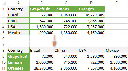
Suppose you have dataset similar to what you see in the upper part of the graphics below. The country names are organized in columns, but the list of countries is too long, so we'd better change columns to rows for the table to fit within the screen:
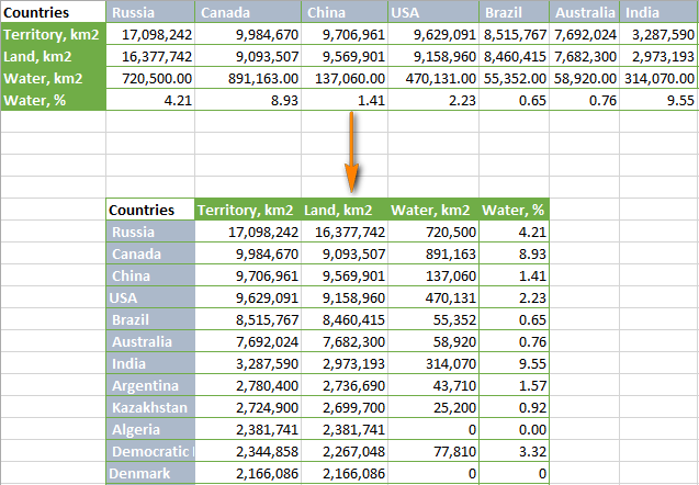
To switch rows to columns in Excel, perform these steps:
- Select the original data. To quickly select the whole table, i.e. all the cells with data in a spreadsheet, press Ctrl + Home and then Ctrl + Shift + End.
- Copy the selected cells either by right clicking the selection and choosing Copy from the context menu or by pressing Ctrl + C.
- Select the first cell of the destination range.
Be sure to select a cell that falls outside of the range containing your original data, so that the copy areas and paste areas do not overlap. For example, if you currently have 4 columns and 10 rows, the converted table will have 10 columns and 4 rows.
- Right click the destination cell and choose Paste Special from the context menu, then select Transpose.
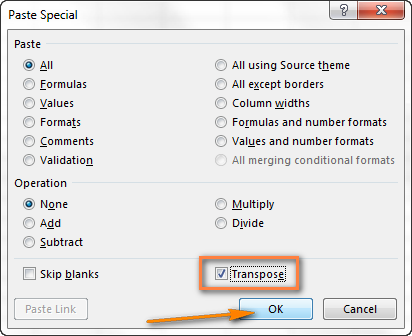
For more information, please see How to use Paste Special in Excel.
Note. If your source data contain formulas, be sure to properly use relative and absolute references depending on whether they should be adjusted or remained locked to certain cells.
As, you have just seen, the Paste Special feature lets you perform row to column (or column to row) transformations literally in a few seconds. This method also copies the formatting of your original data, which adds one more argument in its favor.
However, this approach has two drawbacks that prevent it from being called a perfect solution for transposing data in Excel:
- It is not well suited for rotating fully-functional Excel tables. If you copy the whole table and then open the Paste Special dialog, you will find the Transpose option disabled. In this case, you need either to copy the table without column headers or convert it to a range first.
- Paste Special > Transpose does not link the new table with the original data, so it is well suited only for one-time conversions. Whenever the source data change, you'd need to repeat the process and rotate the table anew. No one would want to waste their time on switching the same rows and columns over and over again, right?
How to transpose a table and link it to the original data
Let's see how you can switch rows to columns using the familiar Paste Special technique, but connect the resulting table to the original dataset. The best thing about this approach is that whenever you change the data in the source table, the flipped table will reflect the changes and update accordingly.
- Copy the rows you want to convert to columns (or columns to be changed to rows).
- Select an empty cell in the same or another worksheet.
- Open the Paste Special dialog, as explained in the previous example and click Paste Link in the lower left-hand corner:
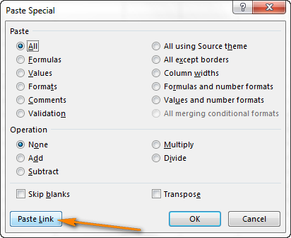
You will have a result similar to this:
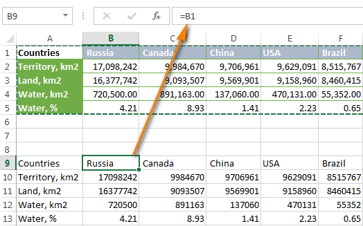
- Select the new table and open Excel's Find and Replace dialog (or press Ctrl + H to get to the Replace tab straight away).
- Replace all "=" characters with "xxx" or any other character(s) that does not exist anywhere in your real data.
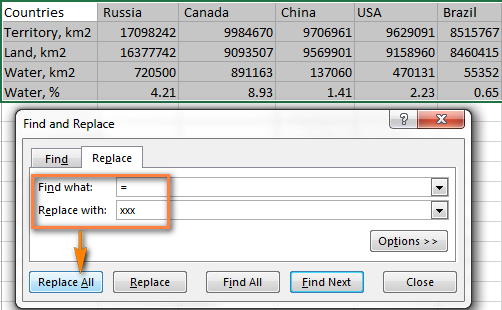
This will turn your table into something a bit scary, as you see in the screenshot below, but don't panic, just 2 more steps, and you'll achieve the desired result.

- Copy the table with "xxx" values, and then use Paste Special > Transpose to flip columns to rows
- Finally, open the Find and Replace dialog one more time to reverse the change, i.e. replace all "xxx" with "=" to restore the links to the original cells.
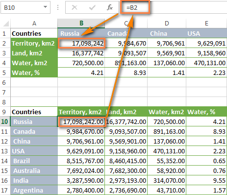
This is a bit long but elegant solution, isn't it? The only drawback of this approach is that the original formatting gets lost in the process and you will need to restore it manually (I'll show you a quick way to do this further on in this tutorial).
How to transpose in Excel using formulas
A quicker way to dynamically switch columns to rows in Excel is by using TRANSPOSE or INDEX/ADDRESS formula. Like the previous example, these formulas also keep the connections to the original data but work a bit differently.
Change rows to columns in Excel using TRANSPOSE function
As its name suggests, the TRANSPOSE function is specially designed for transposing data in Excel:
In this example, we are going to convert another table that lists U.S. states by population:

- Count the number of rows and columns in your original table and select the same number of blank cell, but in the other direction.
For example, our sample table has 7 columns and 6 rows, including headings. Since the TRANSPOSE function will change columns to rows, we select a range of 6 columns and 7 rows.
- With the empty cells selected, type this formula:
=TRANSPOSE(A1:G6)
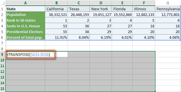
- Since our formula needs to be applied to multiple cells, press Ctrl + Shift + Enter to make it an array formula.
Voilà, the columns are changed to rows, exactly as we wanted:

Advantages of TRANSPOSE function:
The main benefit of using the TRANSPOSE function is that the rotated table retains the connection to the source table and whenever you change the source data, the transposed table will change accordingly.
Weaknesses of TRANSPOSE function:
- The original table formatting is not saved in the converted table, as you see in the screenshot above.
- If there are any empty cells in the original table, the transposed cells will contain 0 instead. To fix this, use TRANSPOSE in combination with the IF function as explained in this example: How to transpose without zeros.
- You cannot edit any cells in the rotated table because it is very much dependent on the source data. If you try to change some cell value, you will end up with the "You cannot change part of an array" error.
Wrapping up, whatever good and easy-to-use the TRANSPOSE function is, it certainly lacks flexibility and therefore may not be the best way to go in many situations.
For more information, please see Excel TRANSPOSE function with examples.
Convert row to column with INDIRECT and ADDRESS functions
In this example, will be using a combination of two functions, which is a little bit tricky. So, let's rotate a smaller table so can better focus on the formula.
Suppose, you have data in 4 columns (A - D) and 5 rows (1 - 5):

To have columns switched to rows, do the following:
- Enter the below formula in the left most cell of the destination range, say A7, and press the Enter key:
=INDIRECT(ADDRESS(COLUMN(A1),ROW(A1))) - Copy the formula rightward and downwards to as many rows and columns as needed by dragging the a small black cross in the lower right hand corner of the selected cells:
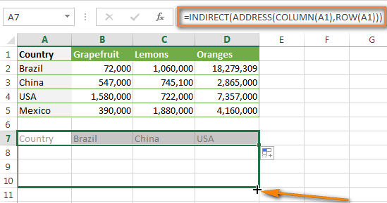
That's it! In your newly created table, all of the columns are switched to rows.
If your data starts in some row other than 1 and column other than A, you will have to use a bit more complex formula:
=INDIRECT(ADDRESS(COLUMN(A1) - COLUMN($A$1) + ROW($A$1), ROW(A1) - ROW($A$1) + COLUMN($A$1)))
Where A1 is the top-left-most cell of your source table. Also, please mind the use of absolute and relative cell references.
However, the transposed cells look very plain and dull, compared to the original data:

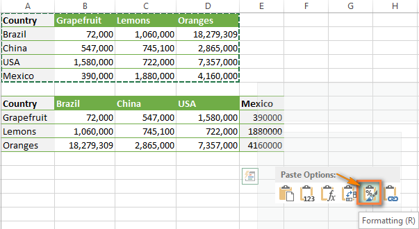
But don't get disappointed, this problem can be easily fixed. To restore the original formatting, here's what you do:
- Copy the original table.
- Select the resulting table.
- Right click the resulting table and choose Paste Options > Formatting.
Advantages: This formula provides a more flexible way to turn rows to columns in Excel. It allows making any changes in the transposed table because you use a regular formula, not an array formula.
Shortcomings: I can see only one - the formatting of the ordinal data is lost. Though, you can quickly restore it, as shown above.
How this formula works
Now that you know how to use the INDIRECT / ADDRESS combination, you may want to get the insight of what the formula is actually doing.
As its name suggests, the INDIRECT function, is used to indirectly reference a cell. But the real power of INDIRECT is that it can turn any string into a reference, including a string that you build up using other functions and the values of other cells. And this is exactly what we are going to do. If you are following up to this, you will understand all the rest with ease : )
As you remember, we have used 3 more functions in the formula - ADDRESS, COLUMN and ROW.
The ADDRESS function obtains the cell address by the row and column numbers you specify, respectively. Please remember the order: first - row, second - column.
In our formula, we supply the coordinates in the reverse order, and this is what actually does the trick! In other words, this part of the formula ADDRESS(COLUMN(A1),ROW(A1)) swaps rows to columns, i.e. takes a column number and changes it to a row number, then takes a row number and turns it to a column number.
Finally, the INDIRECT function outputs the rotated data. Nothing dreadful at all, is it?
Transpose data in Excel using VBA macro
To automate the conversion of rows to columns in Excel, you can use the following macro:
To add a macro to your worksheet, please follow the guidelines described in How to insert and run VBA code in Excel.
Note. Transposing with VBA, has a limitation of 65536 elements. In case your array exceeds this limit, the extra data will be silently cast away.
How to use the macro to convert row to column
With the macro inserted in your workbook, perform the below steps to rotate your table:
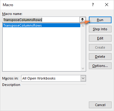
- Open the target worksheet, press Alt + F8, select the TransposeColumnsRows macro, and click Run.
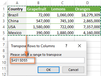
- Select the range where you want to switch rows and columns and click OK:
- Select the upper left cell of the destination range and click OK:
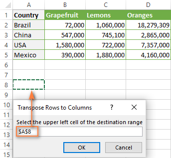
Enjoy the result :)
Switch columns and rows with the Transpose tool
If you need to perform row to column transformations on a regular basis, you may actually be looking for a faster and simpler way. Luckily, I have such a way in my Excel, and so do other users of our Ultimate Suite :)
Let me show you how to switch rows and columns in Excel literally in a couple of clicks:
- Select any single cell within your table, go to the Ablebits tab > Transform group, and click the Transpose button.
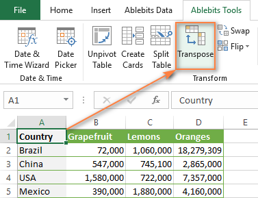
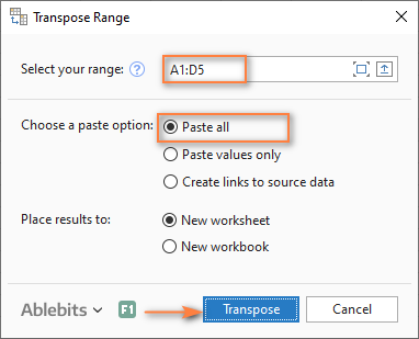
- The default settings work fine in most case, so you simply click Transpose without changing anything.
If you'd like to Paste values only or Create links to source data to force the rotated table to update automatically with every change you make to the original table, select the corresponding option.
Done! The table is transposed, the formatting is preserved, no further manipulations are needed:

If you are curious to try this and 70+ other professional tools for Excel, I invite you to download a trial version of our Ultimate Suite. Thank you for reading and I hope to see you on our blog next week!
 by
by
74 comments
Is there any way to do transpose at a time for multiple columns to rows for all sheets in workbook
It's nice your work but if you are going to change the size of your table you need to be very careful with these procedures because you can confuse and get another result that you don't want.
Take care all of you.
I have a large spreadsheet with close to 5000 rows.
Columns are:
Col1 Col2 Col3 Col4 Col5 Email1 Email2 Email3 Email4 Email5 Email6 Email7
I need to repeat columns 1-5 seven times in order to show each email on a separate row.
So it would like this:
Col1 Col2 Col3 Col4 Col5 Email1
Col1 Col2 Col3 Col4 Col5 Email2
Col1 Col2 Col3 Col4 Col5 Email3
Col1 Col2 Col3 Col4 Col5 Email4
Col1 Col2 Col3 Col4 Col5 Email5
Col1 Col2 Col3 Col4 Col5 Email6
Col1 Col2 Col3 Col4 Col5 Email7
Thanks in advance for your help.
no takers?
I believe you could do this with Query Editor.
1. Open your worksheet in query editor
2. Open the transform tab
2. Make sure headers are correct. You may have to select "use first row as headers"
3. Select all columns that you want to stack into one column (cntr+shft)
4. Select to unpivot table. This should do the trick.
Best answer
Is there a fast way to convert or change the files in 1 row ex row a1 b1 c1 d1 e1 f1 to 1 column exp A1 A2 A3 A4 A5 A6
Use the tutorial from this very article, make sure that the ranges don't overlap when you're trying to transpose.
Or, you can use our add-in.
One Order No. has 4 different sku and 3rd coloumn signifies the quantity of units ordered.. Blank space in first column represents that all sku s belong to order no in the above row. This is what I have:
No sku Qty
200090505 DO-NANO-CABLE-WRAP-TEAL 2
DO-PICO-CABLE-WRAP-TAN 2
DO-SMALL-CABLE-WRAP-TEAL 2
DO-TINY-CABLE-WRAP-BEIGE 2
200090494 BRAINSTO-PPS-PLN-NTBKA5 1
DO-SMALL-CABLE-WRAP-BEIGE 1
This is How I want Basically Transpose it in 1 single row: All sku's in 1 single row adjacent to the order:
Column A B C D E F G H I
Order200090505 SKU QTY SKU QTY SKU QTY SKU QTY
Order200090494 SKU QTY SKU QTY
In excel, how can I transpose data in vertical column into 4 columns and 2 rows because these data pertain to 2 days?
The raw data are the following:
Dec 12 8:15
12:00
1:00
5:00
Dec 13 8:00
12:15
1:00
5:15
I want it to look like this:
12/12/2016 8:15 12:00 1:00 5:00
12/13/2016 8:00 12:15 1:00 5:15
Thank you so much. This helped me a lot.
My data is in the below format.
Type 1/1/2016 1/2/2016 1/3/2016......
A a b g
B g a b
C b g a
I want to change it to the below format:-
Type Date Series
A 1/1/2016 a
B 1/1/2016 g
C 1/1/2016 b
A 1/2/2016 b
B 1/2/2016 a
C 1/2/2016 g
and so on.
I have data for more than 6 months and 35 rows each.
Is there any way I can transpose the data in this format?
Thanks,
Smitha
C
Awesome Article. Thank you so much!
Why do you say "You always need to use absolute references in the Transpose function" -- ? It seems to work just fine without the "$" signs. If I move the source cells, the transposed cells stay the same. If I move the transposed cells, they still stay as is.
Have multiple data lines for same person (not everyone) with multiple values on each line and be a flat figure or a % and would like to move to columns and end up with 1 line for all.
Retirement spreadsheet: the attributes that were created in the HR database was not done in a hierarchy form so each of the below are unique lines.
Roth flat
Roth %
Traditional flat
Traditional %
Partner flat
Partner %
Catch up
Partner catch-up
Is there a simple way to move these into columns?
Hello, Judy,
Looks like you need a VBA script for your task. Sorry, we cannot help you with it.
I want to stack multiple Columns in a column but don't know how??
Hi Svetlana
I wan to transpose row to column and skip the blank cells..
The row could be contain hundred cells,should be transpose to one column avoid the blank.
1-4-0-5- -0-6- -8
BECOME
1
4
0
5
0
6
8
PLS HELLP ME TO MAKE IT WORK..in VBA or Formula
THANKS
You can use wrap text here to get all values in one cell.
=CONCATENATE(H9,
,"
",
I9)
The transpose function = amaze balls!!!!
Thank you
"If your data starts in some row other than 1 and column other than A, simply replace A1 in the formula with a reference to your top-right-most cell."
Not true. It doesn't work with other than A1.
Hi Sandy,
Oops, you are right, it does not work.
The formula for other rows and columns is not so obvious:
=INDIRECT(ADDRESS(COLUMN(A1)-COLUMN($A$1)+ROW($A$1),ROW(A1)-ROW($A$1)+COLUMN($A$1)))
Where A1 is the top-right-most cell of your source table.
Thanks for pointing this out!
thank you so much. nice
I have a problem in need of a solution.
I have columnar data like this
Type1 Type2
ann bob
bob chris
chris john
sue
How do I turn this into a data format presented like this
Type1 Type2
ann X
bob x x
chris x x
john X
sue X
Of course, there are many types and hundreds of names.
Create a pivot table. Use the peoples' names as the "Row". Then select the data you wish to count in the "Values". Make sure that the the value type is either "Sum" or "Count", depending on what you're looking to do with the data.
Aw, this was a really nice post. In idea I would like to put in writing like this additionally
good job
This is brilliant. Thanks so much. You saved me hours and hours of time.
Thank you very much! I'm really glad to know this article was helpful to you.