In this tutorial, you will find a handful of advanced formula examples that demonstrate how to use Excel's VLOOKUP and SUM or SUMIF functions to look up and sum values based on one or several criteria.
Are you trying to create a summary file in Excel that will identify all instances of one particular value, and then sum other values that are associated with those instances? Or, do you need to find all values in an array that meet the condition you specify and then sum the related values from another worksheet? Or maybe you are faced with a more concrete challenge, like looking through a table of your company invoices, identifying all invoices of a particular vendor, and then summing all the invoice values?
The tasks may vary, but the essence is the same - you want to look up and sum values with one or several criteria in Excel. What kind of values? Any numeric values. What sort of criteria? Any : ) Starting from a number or reference to a cell containing the right value, and ending with logical operators and results returned by Excel formulas.
So, does Microsoft Excel have any functionality that can help with the above tasks? Of course, it does! You can work out a solution by combining Excel's VLOOKUP or LOOKUP with SUM or SUMIF functions. The formula examples that follow below will help you understand how these Excel functions work and how to apply them to real data.
Please note, these are advanced examples that imply you are familiar with the general principles and syntax of the VLOOKUP function. If not, the first part of our VLOOKUP tutorial for beginners is certainly worth your attention - Excel VLOOKUP syntax and general usages.
Excel VLOOKUP and SUM - find the sum of matching values
If you work with numerical data in Excel, quite often you have not just to extract associated values from another table but also sum numbers in several columns or rows. To do this, you can use a combination of the SUM and VLOOKUP functions as demonstrated below.
Source data:
Suppose, you have a product list with sales figures for several months, a column per each month. The source data is on the sheet named Monthly Sales:

Now, you want to make a summary table with the total sales for each product.
The solution is to use an array in the 3rd parameter (col_index_num) of the Excel VLOOKUP function. Here is a generic formula:
As you see, we use an array constant in the third argument to perform several lookups within the same VLOOKUP formula in order to get the sum of values in columns 2,3 and 4.
And now, let's adjust this combination of VLOOKUP and SUM functions for our data to find the total of sales in columns B - M in the above table:
=SUM(VLOOKUP(B2, 'Monthly sales'! $A$2:$M$9, {2,3,4,5,6,7,8,9,10,11,12,13}, FALSE))
Important! Since you are building an array formula, be sure to hit Ctrl + Shift + Enter instead of a simple Enter keystroke when you finished typing. When you do this, Microsoft Excel encloses your formula in curly braces like this:
{=SUM(VLOOKUP(B2, 'Monthly sales'!$A$2:$M$9, {2,3,4,5,6,7,8,9,10,11,12,13}, FALSE))}
If you press the Enter key as usual, only the first value in the array will get processed, which will produce incorrect results.
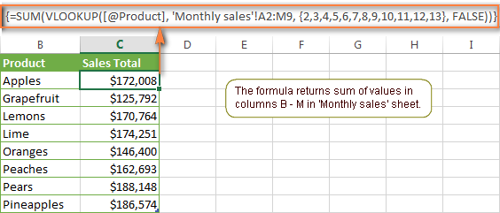
Tip. You may be curious why the formula displays [@Product] as the lookup value in the screenshot above. This is because I converted my data to table (Insert tab > Table). I find it very convenient to work with fully-functional Excel tables and their structured references. For example, when you type a formula into one cell, Excel automatically copies it across the entire column and in this way saves you a few precious seconds :)
As you see, using the VLOOKUP and SUM functions in Excel is easy. However, this is not the ideal solution, especially if you are working with big tables. The point is that using array formulas may adversely affect the workbook's performance since each value in the array makes a separate call of the VLOOKUP function. So, the more values you have in the array and the more array formulas you have in your workbook, the slower Excel works.
You can bypass this problem by using a combination of the INDEX and MATCH functions instead of SUM and VLOOKUP, and I will show you a few formula examples in the next article.
Download this VLOOKUP and SUM sample
How to perform other calculations with Excel VLOOKUP function
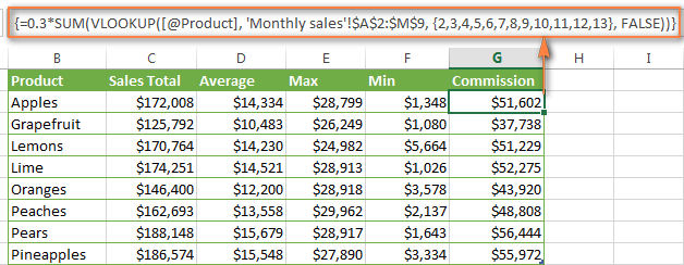
A moment ago we discussed an example of how you can extract values from several columns in the lookup table and calculate the sum of those values. In the same fashion, you can perform other mathematical calculations with the results returned by the VLOOKUP function. Here are a few formula examples:
| Operation | Formula example | Description |
|---|---|---|
| Calculate average | {=AVERAGE(VLOOKUP(A2, 'Lookup Table'$A$2:$D$10, {2,3,4}, FALSE))} | The formula searches for the value of cell A2 in 'Lookup table' and calculates the average of values in columns B,C and D in the same row. |
| Find maximum value | {=MAX(VLOOKUP(A2, 'Lookup Table'$A$2:$D$10, {2,3,4}, FALSE))} | The formula searches for the value of cell A2 in 'Lookup table' and finds the max value in columns B,C and D in the same row. |
| Find minimum value | {=MIN(VLOOKUP(A2, 'Lookup Table'$A$2:$D$10, {2,3,4}, FALSE))} | The formula searches for the value of cell A2 in 'Lookup table' and finds the min value in columns B,C and D in the same row. |
| Calculate % of sum | {=0.3*SUM(VLOOKUP(A2, 'Lookup Table'$A$2:$D$10, {2,3,4}, FALSE))} | The formula searches for the value of cell A2 in 'Lookup table', sums values in columns B,C and D in the same row, and then calculates 30% of the sum. |
Note. Since all of the above formulas are array formulas, remember to press Ctrl+Shift+Enter to enter them correctly in a cell.
If we add the above formulas to the 'Summary Sales' table from the previous example, the result will look similar to this:
Download this VLOOKUP calculations sample
LOOKUP AND SUM - look up in array and sum matching values
In case your lookup parameter is an array rather than a single value, the VLOOKUP function is of no avail because it cannot look up in data arrays. In this case, you can use Excel's LOOKUP function that is analogues to VLOOKUP but works with arrays as well as with individual values.
Let's consider the following example, so that you can better understand what I'm talking about. Suppose, you have a table that lists customer names, purchased products and quantity (Main table). You also have a second table containing the product prices (Lookup table). Your task is to make a formula that finds the total of all orders made by a given customer.
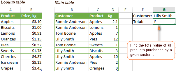
As you remember, you cannot utilize the Excel VLOOKUP function since you have multiple instances of the lookup value (array of data). Instead, you use a combination of SUM and LOOKUP functions like this:
=SUM(LOOKUP($C$2:$C$10,'Lookup table'!$A$2:$A$16,'Lookup table'!$B$2:$B$16)*$D$2:$D$10*($B$2:$B$10=$G$1))
Since this is an array formula, remember to press Ctrl + Shift + Enter to complete it.
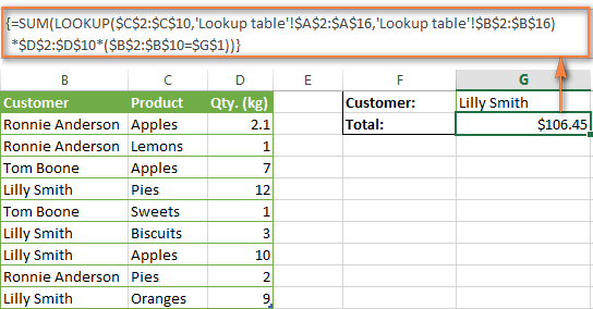
And now, let's analyses the formula's ingredients so that you understand how each of the functions works and can to tweak it for your own data.
We'll put aside the SUM function for a while, because its purpose is obvious, and focus on the 3 components that are multiplied:
LOOKUP($C$2:$C$10,'Lookup table'!$A$2:$A$16,'Lookup table'!$B$2:$B$16)This LOOKUP function looks up the goods listed in column C in the main table, and returns the corresponding price from column B in the lookup table.
$D$2:$D$10This component returns quantity of each product purchased by each customer, which is listed in column D in the main table. Multiplied by the price, which is returned by the LOOKUP function above, it gives you the cost of each purchased product.
$B$2:$B$10=$G$1This formula compares the customers' names in column B with the name in cell G1. If a match is found, it returns "1", otherwise "0". You use it simply to "cut off" customers' names other than the name in cell G1, since all of us know that any number multiplied by zero is zero.
Because our formula is an array formula it iterates the process described above for each value in the lookup array. And finally, the SUM function sums the products of all multiplications. Nothing difficult at all, it is?
Note. For the LOOKUP formula to work correctly you need to sort the lookup column in your Lookup table in ascending order (from A to Z). If sorting is not acceptable on your data, check out an awesome SUM / TRANSPOSE formula suggested by Leo.
Download this LOOKUP and SUM sample
VLOOKUP and SUMIF - look up & sum values with criteria
Excel's SUMIF function is similar to SUM we've just discussed in the way that it also sums values. The difference is that the SUMIF function sums only those values that meet the criteria you specify. For example, the simplest SUMIF formula =SUMIF(A2:A10,">10") adds the values in cells A2 to A10 that are larger than 10.
This is very easy, right? And now let's consider a bit more complex scenario. Suppose you have a table that lists the sales persons' names and ID numbers (Lookup_table). You have another table that contains the same IDs and associated sales figures (Main_table). Your task is to find the total of sales made by a given person by their ID. At that, there are 2 complicating factors:
- The mail table contains multiple entries for the same ID in a random order.
- You cannot add the "Sales person names" column to the main table.
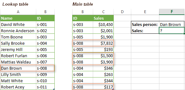
And now, let's make a formula that, firstly, finds all sales made by a given person, and secondly, sums the found values.
Before we start on the formula, let me remind you the syntax of the SUMIF function:
range- this parameter is self-explanatory, simply a range of cells that you want to evaluate by the specified criteria.criteria- the condition that tells the formula what values to sum. It can be supplied in the form of a number, cell reference, expression, or another Excel function.sum_range- this parameter is optional, but very important to us. It defines the range where the corresponding cells' values shall be added. If omitted, Excel sums the values of cells that are specified in the range argument (1st parameter).
Keeping the above info in mind, let's define the 3 parameters for our SUMIF function. As you remember, we want to sum all the sales made by a given person whose name is entered in cell F2 in the main table (please see the image above).
- Range - since we are searching by sales person ID, the range parameter for our SUMIF function is column B in the main table. So, you can enter the range B:B, or if you convert you data to a table, you can use the column's name instead:
Main_table[ID] - Criteria - because we have sales persons' names in another table (lookup table), we have to use the VLOOKUP formula to find the ID corresponding to a given person. The person's name is written in cell F2 in the main table, so we look it up using this formula:
VLOOKUP($F$2,Lookup_table,2,FALSE)Of course, you could enter the name in the lookup criteria of your VLOOKUP function, but using an absolute cell reference is a better approach because this creates a universal formula that works for any name input in a given cell.
- Sum range - this is the easiest part. Since our sales numbers are in column C named "Sales", we simply put
Main_table[Sales].Now, all you need is to assemble the formula's parts and your SUMIF + VLOOKUP formula is ready:
=SUMIF(Main_table[ID], VLOOKUP($F$2, Lookup_table, 2, FALSE), Main_table[Sales])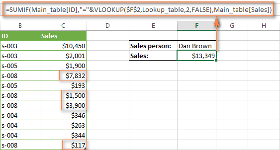
Download this VLOOKUP and SUMIF sample
Formula-free way to do vlookup in Excel
Finally, let me introduce you to the tool that can look up, match and merge your tables without any functions or formulas. The Merge Tables tool included with our Ultimate Suite for Excel was designed and develop as a time-saving and easy-to-use alternative to Excel's VLOOKUP and LOOKUP functions, and it can be very helpful both to beginners and advanced users.
Instead of figuring out formulas, you simply specify your main and lookup tables, define a common column or columns, and tell the wizard what data you want to fetch.
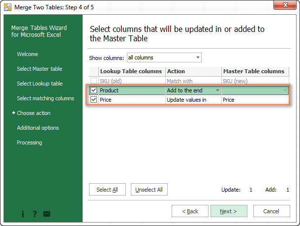
Then you allow the wizard a few seconds to look up, match and deliver you the results. If you think this add-in may prove helpful in your work, you are most welcome to download a trial version by using the below link.
Available downloads
VLOOKUP with SUM and SUMIF - formula examples (.xlsx file)
Ultimate Suite - trial version (.exe file)
 by
by
423 comments
i have some invoices in sheet1 and i want to make a summary with product name and Quantity in sheet2
so please help me to solve this problem detils are
PRODUCT QTY
AREIL 45G 96
AREIL 500G 12
SAFEGUARD 115G W 72
SAFEGUARD 115G L 144
H&S 200ML CC 6
H&S 200ML B 12
PANTENE 90ML SS 24
PRODUCT QTY
JELLETT BLUE 2+ 24
MACH 3 RAZOR 3
AREIL 45G 24
AREIL 1000G 6
SAFEGUARD 115G W 144
AREIL 500G 6
What formula can return all possible combinations of numbers that add up to a given total. For example, let's say the given total is the number 137. Which combinations of numbers would add up to 137? To make this more interesting, no number can be repeated, and no more than 5 numbers can ever be used in one single try. So 7+35+45+49+1=137, but many more combination do as well. Thank you.
Hello Steven,
It is an interesting task, but I'm afraid we can't calculate it using formulas. It would be useful to find a Maths student with a good knowledge of VBA :)
Hi Everyone and anyone, pls. if you know the formula to the given equation pls. share the answer... Thanks
I have 3 sheets in each three sheets in column A is there are common and different no. how do i get these no. but NOT get repeated in my another "final" sheet,
Second, i want to get the sum of each 3 sheets for column A representing in different cells data to Final sheet.
So, for First result i tried =IFERROR(VLOOKUP('1st Month'!$D4,'2nd Month'!D4:D22,1,0),IFERROR(VLOOKUP('2nd Month'!$D4,'3rd Month'!D4:D23,1,0),IFERROR(VLOOKUP('1st Month'!$D4,'3rd Month'!D4:D25,1,0),"0"))) formula and not sure if this right.
for second Result i Tried = SUMPRODUCT(SUMIF(INDIRECT(""&test&"''!$D$4:$D$19"),$D4,INDIRECT(""&"'!$I$4:$I$19")), Pls Help me in getting the expected answer. Thanks
Hello Rahul,
What concerns your first task, the easiest way would be copying all column A values from three sheets into your final sheet, removing duplicates, and then applying the VLOOKUP formula.
As for summing the corresponding values from three sheets, it sounds like data consolidation is the best option for you. Please see this blog post for detailed steps:
How to consolidate data from multiple worksheets
Hi Maria,
i have 3 sheets in each three sheets column A is the common and different no. how do i get these no. not get repeated in my another "final" sheet.
Second, i want to get the sum of each 3 sheets column A representing data to Final sheet.
So, for First result i tried =IFERROR(VLOOKUP('1st Month'!$D4,'2nd Month'!D4:D22,1,0),IFERROR(VLOOKUP('2nd Month'!$D4,'3rd Month'!D4:D23,1,0),IFERROR(VLOOKUP('1st Month'!$D4,'3rd Month'!D4:D25,1,0),"0"))) formula and not sure if this right.
for second Result i Tried = SUMPRODUCT(SUMIF(INDIRECT(""&test&"''!$D$4:$D$19"),$D4,INDIRECT(""&"'!$I$4:$I$19")), Pls Help me in getting the expected answer. Thanks
Sir
I need help about I have Two Spreed Sheet of Excel I want If Sheet1 Cell F1 is equal to or Greater than 19 then Copy Sheet1 Cell A1:D1 and paste the same in Sheet2 A1:D1 please help me for this formula i have urgently required
Hello Nisar Ahmad,
Please enter the formula below into cell A1 of Sheet 2:
=if(Sheet1!$F$1>=19, Sheet1!A$1,””)
Then copy the formula to all cells in the row: B1 to D1.
Hi Jim,
I have emailed you the excel sheet with the solution which would be more clear to you. Moreover I am not able to attach the excel file in this blog.
Regards,
Ramki
Hello Ramki,
I'm sorry, but we can't seem to find your email. Could you please make sure you sent it to support@ablebits.com? Please include the name of the blog post and the number of your comment.
Good afternoon!
I have a task in which I will be referring to two sheets. On the first sheet, I will have a name column (A1:A200) and a quantity column (B1:B200).
On the second sheet, I will also have a name column and a quantity column, A and B respectively. My task is to search each name of sheet1!A1:A200 for a matching name on sheet2! Where there is a name match, I need to have the quantities added together. I hope you can assist me!
thank you!
Hi
I have managed to get a sumif and combine it with a vlookup and that seems to give me the answers I need, but what I want to do is know when the values I've added reach a defined range of 335-395, and then return me the cell which falls in that range
Any suggestions would be great!!
Thanks
Hello, Helen,
To help you better, we need a sample table with your data in Excel. You can email it to support@ablebits.com. Please add the link to this article and your comment number.
Below the letter A are the number 15, 23 and 15.
Below the letter B are the number 18, 13 and 20.
Below the letter C are the number 50, 19 and 30.
Thanks.
Hello, Dung,
You need an array formula:
=SUM(IF(ISERROR(OFFSET(A2:C6, -1, 0)), 0, IF((OFFSET(A2:C6, -1, 0))="A", 1, 0) ) * (IF(ISNUMBER(A2:C6), A2:C6, 0)))
Your data are in A1:C6. Use the same formula for B and C, just change ="A" correspondingly.
Make sure you press CTRL+SHIFT+ENTER after entering the formula.
Hi Svetlana,
I have those simple data in excel. How can I sum all the number right below letter A, or B or C if the staggering on in order in Excel. Thanks.
A B C
15 18 50
B C A
13 19 23
C A B
30 15 20
hi
I have a expense chart in which I2 to I25 have list of categories.
A is for seriel number
B is for date
C is for amount of expense
D for category
E is for mode of payment
F is for expense category
G is for commulative total
Now I want to make a separate sheet which can show all the list of categories and after each category there should be total of expenses done in that category.
Kindly help me how to do. I wantto make separate sheet for this.
Regards
Gk
Hello, Gk,
Please check if the Split Table add-in can help with your task:
https://www.ablebits.com/excel-split-table/index.php
Hello all,
kindly help
i am making result card of students in ms excel.
i need to add marks obtained and total marks
but
there is a restriction
there are total 7 subjects with different total marks e.g.
English (100), History (100), Mathematics (85), Chemistry (85), Physics (75), Computer (75) and Biology (85).
Rest of subjects are compulsory for students except Biology and Computer
Those who attempt computer will not be attempting Biology and vice versa
so i need a formula to get total marks sum
example what i want
if ( bio == 0 )
{
sum English+History+Mathematics+Chemistry+Physics+Computer
}
%answer is 520 %
else if (comp == 0)
{
sum English+History+Mathematics+Chemistry+Physics+Biology
}
%answer is 530 %
%In case some is absent from computer or biology paper we need to add total of their respective subjects so %
else if ( Comp == 'A' )
{
sum English+History+Mathematics+Chemistry+Physics+Computer
}
else if (Bio == 'A')
{
sum English+History+Mathematics+Chemistry+Physics+Biology
}
waiting for a favourable response
Hello, Yousaf,
To help you better, we need a sample table with your data in Excel. You can email it to support@ablebits.com. Please add the link to this article and your comment number.
If I have a table with the following:
FP2000 30,000
FP2001 45,000
FP2000 50,000
What formula would I use to grab the repeating "FP's" and then sum them up, without using a pivot table?
Hello , i would like to know which formula to use if i have a colum of values and i want to point out the values that would add to a specific number , for example ;
D
1
2
4
8
23
19
7
And out of that range i would do a formula that would tell me which will add up to 29.
Hello, Nicolas,
For us to be able to assist you better, please send us a small sample table with your data in Excel to support@ablebits.com.
Am trying to sum column m where last 6 characters in column a is in month of dec-15, but I only seem to be summing the first occurrance of dec-15 in column a. Any ideas? Thanks for looking.
=SUMIFS(Fees!M2:M110,Fees!A2:A110,RIGHT(TEXT(A58,"mmm-yy"),6))
Hello, Steve,
Please try this array formula:
=SUM((M1:M110) *(RIGHT(TEXT(A1:A110, "mmm-yy"), 6)="Dec-15"))
Make sure you press CTRL + SHIFT + ENTER after entering the formula.
Can the VLOOKUP function be used in conjunction with the SUM function to replace the sum range function argument?
Hello, Gary,
To be able to assist you we need to see your data. Please give us an example.
s-003 $10,450 Sales person: Dan Brown
s-003 $2,001 Sales: $13,349
s-005 $1,900
s-008 $7,832
s-005 $193
s-008 $1,500
s-008 $3,900
s-004 $346
s-004 $263
s-004 $344
s-008 $117
same type but different excell
Hai,
Please send how to calculate excel to excel sumif+vlookup
total qty required in one format
Svetlana
From your about example, {=SUM(VLOOKUP(B2, 'Monthly sales'!$A$2:$M$9, {2,3,4,5,6,7,8,9,10,11,12,13}, FALSE))}, is there anyway to replace the hard coded set {2,3,4,5,6,7,8,9,10,11,12,13} with a cell reference or set of cell reference like {A6,B6,C6,D6}? I would like to not have to edit the set reference every time I change or add a new section to my workbook.
Thanks for the advice!!
Hello, Dennis,
Sorry, looks like this is not possible.
I have a table of 3 columns: Course, Credit and Category:
Course Credits Category
10 3 GE
20 3 GE
22 3 GE
40 3 GE
56 3 Surveys
71 3 Lower Division CW
I have another worksheet where I am entering the courses per instructor and totaling the units
so for Fall 15 semester teacher teaches 3 courses and it totals the units
Cindy 22 40 56 9 units
Bill 71 56 40 9 units
I used a vlookup to calculate the units based on which course was entered and total it by semester by instructor. That works fine.
I want to now total the categories for each semester
Categories
GE
Surveys
Lower Division
It should look up the category associated with the course (Above table course 10 is a GE Category) and count the instances where it finds a course that falls into the GE Category.
GE 15 courses
Surveys 10 courses
Lower Division 9 courses
Any help you can give me will greatly appreciated
Hello Debbie,
Can you please send me your sample workbook at support@ablebits.com?
Dear i have following example data of 3 different clients. Now if i want to sum "Apple", "Orange" etc. then what kind of formula should be use. plz guide.
Ahmed & CO =
APPLE 5 2 3 4
ORANGE 4 1 2 3
LEMON 3 4 5 5
COCONUT 2 1 3 4
Sharif & CO =
ORANGE 4 2 4 2
APPLE 6 4 4 5
COCONUT 3 7 4 6
Sharif & CO =
COCONUT 2 4 3 2
ORANGE 4 3 4 2
APPLE 5 3 2 4
Sl No. ItemID Program Category Efforts
1 P001 Interior Design 120
2 P002 Exterior Drawing 40
3 P003 CAE annotation 33
4 P004 Seating Packaging 456
5 P005 Interior Design 22
6 P006 Interior Drawing 55
7 P007 Exterior annotation 6677
8 P008 Exterior Packaging 244
9 P009 Exterior annotation 786
10 P010 CAE Packaging 44
11 P011 CAE Design 245
12 P012 Seating Packaging 9887
13 P013 Exterior Design 54
14 P014 Exterior Drawing 444
Hi Svetlana,
Please help me to get a formula to get the total efforts when program and category in different rows same.
Exampple : from above data
Sl No. 4 & 12 have same program and category, so their sum is 10343.
Hi
I have an expense report that runs chronologically for an entire year. I would like to have a formula that can sum the amounts by month and by item. I.e. Sum all amounts in column X (highlight entire range) that say January in column Y and "Elect. bill" in column Z. Is this even possible?
I have 50000 entries in excel sheet and i have to do page wise totals. Needs to print on dot matrix printer later on. I also need page wise summary of totals.
there are entries like voucher No.s having different transactions. I want to club the total amount against the one voucher No. instead of repeating it. it will save paper. Please help
Thanks
Very good site , very educative
I have a situation similar to the first example on this page, i.e. fruits in multiple rows and months as columns. The formula is great for finding one fruit and adding multiple columns in the array. However, I have the same fruit listed in multiple rows. I need to add the months amounts for each row that the fruit is listed. Is there a way I can do this in a formula without creating a pivot table?
Thanks
I need a formula to update a sales sheet. as i have multiple of contract numbers in one column and each contract has some value that i want to sum. with pivot table it be done however i need a formula. can please advice...
Contract # Status Car Plate # Pymt_Customer
577 Open 7823 1500
586 Open 7827 0
586 Closed 7827 165
584 Open 7822 1500
584 Closed 7822 -1020
577 Closed 7823 -265
i need to add values corresponding to (say) 4th coloumn if values or data in 1st 2nd and 3rd coloumn match.
division name date expense
sales a 20-Jul-15 1
pdtn b 5-Jul-15 2
sales c 10-Jul-15 3
pdtn d 20-Jul-15 4
sales a 5-Jul-15 5
sales a 10-Jul-15 6
sales a 20-Jul-15 7
sales c 10-Jul-15 8
sales c 5-Jul-15 9
pdtn d 20-Jul-15 10
if data of A , B AND C coloumn match then it should do sum total of values in D
for any new unique combination of A,B and C coloumn a new row automatically should be created
I want the result to be like this
sales a 20-Jul-15 8 (1+7)
pdtn b 5-Jul-15 2
sales c 10-Jul-15 11 (3+8)
pdtn d 20-Jul-15 14 (10+4)
sales a 5-Jul 5
sales a 10-Jul 6
sales c 5-Jul-15 9
can someone help me on this. thanks in advance
Hi, Svetlana. I read your article on SUM and VLOOKUP and I practiced some examples about the combination of SUM and VLOOKUP/ INDEX. And I have some questions relating to the first example in above article.
I want to extract the apples' sales figures for 3 months (Jan, Feb, Mar) separately in 3 cells. I choose 3 cells and enter the same array formula:
{=VLOOKUP("apples",'Monthly sales'!$A$2:$M$9, MATCH({"Jan","Feb","Mar"},'Monthly sales'!$A$1:$M$1,0))}
Result of above formula is 3 cells contain sales figures of 3 months.
And I use INDEX formula and receive the same results:
{=INDEX('Monthly sales'!$A$2:$M$9, MATCH("apples",'Monthly sales'! $A$2:$A$9,0),MATCH({"Jan","Feb","Mar"},'Monthly sales'!$A$1:$M$1,0))}
My PROBLEM is:
1- When I use the combination VLOOKUP with SUM and received a correct result as the following:
{=SUM(VLOOKUP("apples",'Monthly sales'!$A$2:$M$9, MATCH({"Jan","Feb","Mar"},'Monthly sales'!$A$1:$M$1,0)))} =$26,189
2- But when I try to combine SUM with INDEX in a similar way, I only receive the apples'sales of Jan:
{=SUM(INDEX('Monthly sales'!$A$2:$M$9, MATCH("apples",'Monthly sales'! $A$2:$A$9,0),MATCH({"Jan","Feb","Mar"},'Monthly sales'!$A$1:$M$1,0)))} =$2,773
- However, when I calculate the apples' sales for all 12 months by using SUM and INDEX (with col_num =0), I receive the correct result.
{=SUM(INDEX('Monthly sales'!$A$2:$M$9, MATCH("apples",'Monthly sales'! $A$2:$A$9,0),0))} =$172,008
Could you please explain for me why the second formula not return the correct result?
I looking forward to receiving your reply. Thank you.
Hi Svetlana,
Need your expertise again!!! I am suppose to make performance meter but can't get the desired results. Please have a look;
Year Month Name leads Matured Conversion%
2015 June Anju 30 2 7%
2015 June Rekha 28 2 7%
2015 June Somya 35 2 6%
2015 July Anju 40 4 10%
2015 July Rekha 35 5 14%
2015 July Somya 45 5 11%
How to get the average of Conversion% based upon extracting data from below selection:
Select [From Month/Year---> to Month/Year] eg; [2015/June--->2015/July]
Select Name eg; Anju
Result should show Average% of selected Name based upon year and month range selected.
I have been trying vlookup, index & match, sumif but didn't get through.
PURCHASE
SL.No GRADE FINISH THIKNESS WIDTH HEIGHT GRAVITY NO COIL QTY
1 304 15.84 0.6 1500 2200 0.000008 1 Yes 15.84
2 316 15.84 0.6 1500 2200 0.000008 1 Yes 15.84
3 321 15.84 0.6 1500 2200 0.000008 1 Yes 15.84
4 309 15.84 0.6 1500 2200 0.000008 1 Yes 15.84
5 LN-1 15.84 0.6 1500 2200 0.000008 1 Yes 15.84
6 LN-4 15.84 0.6 1500 2200 0.000008 1 Yes 15.84
7 200-S 15.84 0.6 1500 2200 0.000008 1 Yes 15.84
8 SA 15.84 0.6 1500 2200 0.000008 1 Yes 15.84
9 430 15.84 0.6 1500 2200 0.000008 1 Yes 15.84
I need the vlookup formula for the above.
you can see in the second coloumn "GRADE" that is the order may apper many times and need to add the vales of grade. Value is in 'QTY' column. pls let me know how I can do the look up formula.
Hi All,
I have two worksheets.
One listing all days against a individual contract e.g.
Contracts Days
1234 1
1234 4
1234 2
1234 9
1235 1
1235 6
1235 0
1235 11
1236 7
1236 2
1236 20
1237 1
1237 7
1237 5
1237 5
and the other where I want to look this days total up for that contract e.g.
Contract Total days
1234 16
1235 18
1236 29
1237 18
What VLOOKUP & SUM formula would I use as column one would not work as it is SUMing rows.
Maybe,you can try using SUMIF function.
Supposing that in Sheet1 the column Contract_number is A2:A16 and column Days is B2:B16 ; in Sheet2 column Contract is A2:A5
In Sheet2 choose ALL cells B2:B5 and enter a same array formula in Formula bar:
=SUMIF('Sheet1'!A2:A16,=A2:A5,'Sheet2'!B2:B16)
Due to it is an array formula and should be ended by Ctrl+Shift+Enter
hi,
I want to add the individual values of each week for all the months in a year for a list of items.
I need these to be calculated automatically in a different sheet. Could you help me out with this.
For example, the main sheet looks something like the below table:
5Jan - 9Jan 12Jan - 16 Jan etc
Opening count 1 2
New 5 7
Closed 4 6
Backlog 2 3
In sheet2:
I need the following result:
Jan
Opening Count 1
New 12
closed 10
Backlog 3
This needs to be done for all 12 months.
Hello,
I am working on an extensive spreadsheet with thousands of loan numbers, names, document types, ID numbers, etc. My issue is that each week, this company will send me a spreadsheet of thousands of loans but could very well be duplicates of the previous week. I cannot simply use the function "remove duplicates" because the loans are always duplicated with each separate document request and if I have one loan repeated 3x because it requires 3 different document types, that function will remove 2 of them and throws everything off. How can I weed out the prior week's loan numbers and simply identify what loans are new to the current weeks' spreadsheet? Sorry to be so longwinded. :-)
Hi,
I have a budget sheet where there is certain budget is allocated in different months under a certain budget heading. And I have a reporting month cell where I have a dropdown box including the names of the month. Now, what I want is to get the result of the sum of the budget of the activity when i respectively change the month. I also want to get the value, if I click the month to march, then i need the cumulative budget value added till march.
Please help
I have a combination of value such as '1/3 in A1, '3/3 in A2 and '3/6 in A3. Is there a way to sum the that are 1+3+3 so that in the cell I would have 7 and the next cell 3+3+6 that would equal to 12? Basically, I need to sum the 1st values of the A1, A2 and A3 and in the other cell 2nd values of the same cells?
Greetings, I am trying to build a workbook that has 3 sheets. One for entry of first last name and ID number as well as a monetary value like a tip. On the second sheet is the summary page where i wanted the table to return the sum of all information by employee id to give me a total of tips for that employee. The third page i had set up as the reference table where i would enter the First last name and ID number. I tried using your example but still cant get it to work.
I have pasted the formula below.
Can you help?
Im also using google documents
={=SUM(Tips!$c$2:$c$30*IF(Tips!$C$2:$C$30=TRANSPOSE(Employee!$c$2:$c$30),TRANSPOSE(Employee!$c$2:$c16),0)*($C$2:$C$2=$I$1))}
hi,
i have a table in my excel file having different Items date wise, eg:-
Date No. Name Item quantity
1/4/15 106 Ab Apple 50
1/4/15 129 Bd Mango 75
1/4/15 235 Jp Mango 39
2/4/15 114 Tk Mango 63
2/4/15 228 Kl Orange 24
3/4/15 0 0 0 0
4/4/15 0 0 0 0
5/4/15 235 Jp Mango 52
5/4/15 106 Ab Orange 28
...
.
.
.
.
and so on date wise, actually i want to monthly date wise quantity in one cell.
which formula i have to use if i need the quantity of Mango for selected date?
eg. if i put a date 1/4/15 and match with item Mango, so that in a one cell the total quantity should be 114.
Hi Svetlana!
I have a column of numbers from which I want the top 10% of the sum of the column to be highlighted. I tried the conditional formatting option. But it doesn't give me a result which is even near 10%.
Hi Mei, we have the same problem! I hope somebody can help!
hi.. im having trouble with my excel..
you see..my proble is like this
qty.-------u/m-------product
2 ------rolls------ thermal paper
5 ------packs------ pandan jelly
4 ------rolls ----- thermal paper
i want to have a summary like this
thermal paper----- 6
pandan jelly -----5
Hi Mei,
Supposing that Qty. is column A and Product is column C, you can use the following SUMIF formula:
=SUMIF(C2:C100, "thermal paper", A2:A100)
thanks!! that helps a lot!!
but there is another one.
example:
qty----u/m----product------amount
2-----packs---12 oz lid----
5-----rolls---thermal paper---
1-----box-----12 oz lid---
what i want is somehow, when i type the qty, u/m and product, it will give like...
thermal paper---6----$
12oz lid (pack)----2-----$
12oz lid (box)-----1-----$
there should be a difference in the price of the per box and per packs... thanks
THANK YOU FOR YOUR WONDER FULL POST. I CAN'T REALLY GET IT RIGHT!!!
BSERVATION
FOR FIND SAME MATCH =VLOOKUP(A:A,A:B,2,FALSE) (MIDLE A:B SHEET TO SHEET UR O)
FOR SUM OF MATCH =SUMIF(A:A,A,B:B) (MIDLE "A" IS OBSERVATION TO FIND)
THIS IS SUM OF ALLLL YOUR POST. YOU CAN MAIL ME IF DOUBT.
ADD SUMIF CRITERIA (MIDDLE AREA) BY SELECT THE CELL YOU WANTED TO SUM.
Thanks Svetlana! Another question, We got the below formula to work, Thanks for the Ctrl+Shift Enter tip.
{=SUM(VLOOKUP("Green",$I$26:$L$28, {2,3,4}, FALSE))}
Jan Feb March
Green 10 40 70
Purple 20 50 80
Yellow 30 60 90
120
However, we could not get the same formula to work for the below table. Help please.
Jan Feb March
Green 10 40 70
Green 20 50 80
Yellow 30 60 90
120
Hi Vladamir,
Both tables seem to be identical. Can you check please?
Hi Svetlana, I copied your formula and my sample data is below. I used the formula, =SUM(VLOOKUP("Aaron",$I$26:$J$28,2,FALSE)) I was expecting 50, but got 30. Help please.
Aaron 30
Aaron 20
Jack 10
30
Hi Vladamir,
Since you are working with a single table, you don't need SUM/VLOOKUP. A simpler SUMIF formula works just fine:
=SUMIF($I$26:$J$28, "aaron", $J$26:$J$28)
Hi,
Is there any possible way to sum data without mentioning "aaron"
I mean automatically it will sum if the Column A duplicated
Hi Vivien,
You can use the following formula:
=SUMIF($A$2:$A$6, $F2, B$2:B$6)
Where A is the currency column in your main table, B is data for 01-Jan, and F is the currency colum in your summary table.
Hi,
I have a huge set of data looks like this:
A B C
1 CCY 01-Jan 02-Jan
2 EUR 1000 500
3 EUR 150 50000
4 USD 2000 480
5 JPY 340000 348212
6 USD 3000 23934
How can I sum data into below format without using pivot table?
01-Jan 02-Jan
EUR
USD
JPY
Thanks.
Vivien
I have a column of 16 cells with a list of upgrades depending upon the unit style. I have a table with the 3 different upgrades levels and the corresponding price. I would like to SUM the total amount of the upgrades in one cell. I thought it should be a sum with vlookup but it's not returning a value. Any suggestions?
When I use this formula it only returns the value from the first cell. It doesn't give me the total from the other cells in the lookup value selection.
{=SUM(VLOOKUP(C40:C55,$A$34:$B$36,2,FALSE))}
Could use some Excel wisdom. I have tried tweaking examples given, but am still struggling. I need to sum data for each month based on a name using 2 tables:
--Table 1--
Jan Feb Mar...
A 5 8 6
B 2 6 9
C 3 5 12
--Table 2--
A Bob Smith
B Nancy Jones
C Bob Smith
Based on the name, I need a cell to sum all the values associated with the name for the month. So, in the example above, given "Bob Smith", the cell would return a value of 8 for January. I tried SUM & VLOOKUP and then MATCH & INDEX combos, and cannot make it work. Can someone kindly advise? Thank you.
Thank you!
Hey,
Please help me how to solve this by using v look up.
01/01/1991 Andy
02/03/1991 Josepf
01/04/1990 John
05/07/1989 Cathy
01/12/1990 Ray
03/08/1990 Edmond
03/07/1988 Steve
03/03/1987 Peter
Want to get the names of the person who born in the year 1990 by using Vlookup.
Thanks