What is PV in Excel? It's a function to calculate present value. This tutorial explains its syntax, shows how to build a correct PV formula for a series of cash flows and a single payment, describes what pitfalls you may encounter and how to overcome them.
Suppose you are thinking about buying an insurance annuity to secure a steady cash flow during your retirement years. Or maybe you consider putting some money in a saving account with a decent annual interest. Whatever it is, you are wondering - is that a good deal? To know it for sure, you need to find the present value of an investment. For this, Microsoft Excel provides the PV function, which stands for "present value".
Excel PV function
PV is an Excel financial function that returns the present value of an annuity, loan or investment based on a constant interest rate. It can be used for a series of periodic cash flows or a single lump-sum payment.
The PV function is available in all versions Excel 365, Excel 2019, Excel 2016, Excel 2013, Excel 2010 and Excel 2007.
The syntax is as follows:
Where:
- Rate (required) - the interest rate per period. If you make yearly payments, indicate an annual interest rate; if you pay monthly, specify a monthly interest rate, and so on.
- Nper (required) - the total number of payment periods for the length of an annuity.
- Pmt (optional) - the amount paid each period. If omitted, it is assumed to be 0, and the fv argument must be included.
- Fv (optional) - the future value of an annuity after the last payment. If omitted, it is assumed to be 0, and the pmt argument must be included.
- Type (optional) - when the payments are to be made:
- 0 or omitted (default) - at the end of a period (regular annuity)
- 1 - at the beginning of a period (annuity due)
5 things you should know about PV function
For the Excel PV function to work correctly in your worksheets, please take into account these usage notes:
- If the fv argument is zero or omitted, pmt must be included, and vice versa.
- The rate argument can be supplied as a percentage or decimal number, e.g. 10% or 0.1.
- Any money that you pay out (outflow) should be represented by a negative number. Any money that you receive (inflow) should be represented by a positive number. For example, when you are investing money into an insurance annuity, use a negative number for pmt. When the insurance company begins making payouts to you, express payments as positive numbers.
- When calculating periodic cash flows, be consistent with the rate and nper units. For instance, if you make 5 yearly payments at a 7% annual interest rate, use 5 for nper and 7% or 0.07 for rate. If you make monthly payments for a period of 5 years, then use 5*12 (a total of 60 periods) for nper and 7%/12 for rate.
- All the arguments must be numeric, otherwise the PV function returns a #VALUE! error.
Basic PV formula in Excel
To get a general idea of how to use the PV function in Excel, let's construct a present value formula in its simplest form.
Suppose you are making regular contributions to build up your savings for retirement. You deposit $500 per period at a 7% interest rate and will do 50 such payments at equal intervals.
To find the present value of the annuity, set up your worksheet in this way:
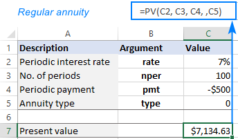
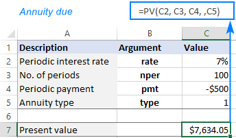
- Periodic interest rate (C2): 7%
- Number of periods (C3): 100
- Payment amount (C4): -500
- Annuity type (C5): 0 (regular annuity) or 1 (annuity due)
The formula to calculate the PV of the investment is:
=PV(C2, C3, C4, ,C5)
If you compare the results of the ordinal annuity (payments are made at the end of the period) and annuity due (payments are made at the beginning of the period), you'll notice that, in the latter case, the present value is higher.
PV of regular annuity:

PV of annuity due:

And here are a few more things to take notice of:
- In this example, the pmt argument is a negative number because we invest the money. If you calculate PV of an annuity that pays to you, then enter pmt as a positive number, and you'll get a negative PV as the result.
- The future value is not used in this calculation, therefore the fv argument is omitted.
- When making a PV formula for monthly cash flows (or other periodic payments such as weekly, quarterly, etc.) remember to convert an annual interest rate to a periodic rate as shown in this example.
You can also look at the problem from another angle. To find the interest rate at which PV is 0, use the IRR function.
How to use PV function in Excel - formula examples
The following examples will give you the insight of how the Excel PV function works in different scenarios, so you could adjust the basic formula for your specific task.
Calculate PV of annuity
Let's say you bought an annuity in which a regular payment of $200 is to be made to the insurance company at the start of every month for the next 10 years. The annuity earns a 9% annual interest compounded monthly. The question is - how much is this annuity worth now?
To begin with, enter all the data in separate cells:
- Annual interest rate (B2): 9%
- Number of years (B3): 10
- Monthly payment (B4): -200
- Annuity type (B5): 1
- Number of periods per year (B6): 12
In this case, the interest rate (rate) and payment (pmt) are for different periods. To do PV right, we need to make a couple of conversions:
To convert an annual interest rate to a periodic rate, divide the annual rate by the number of periods per year:
rate = annual interest rate / no. of periods per year
To get the total number of periods, multiply the annuity term in years by the number of periods per year:
nper = no. of years * no. of periods per year
Since we have a monthly annuity, we can divide and multiply by 12 or by cell B6 in which this number is entered.
The complete PV formula in B8 is:
=PV(B2/B6, B3*B6, B4,, B5)

In a similar manner, you can calculate the present value of a weekly, quarterly or semiannual annuity. For this, simply change the number of periods per year in the corresponding cell:
- Weekly: 52
- Monthly: 12
- Quarterly: 4
- Semiannual: 2
- Annual: 1
Calculate PV of investment based on its future value
In this example, we are going to find the present value of an investment that will pay $50,000 in 5 years, with an annual interest rate of 7%. The goal is to find out how much money we need to invest today to reach the target amount at the end of the investment period.
As usual, we input the annuity data in separate cells:
- Annual interest rate (B2): 7%
- Number of years (B3): 5
- Future value (B4): 50,000
- Annuity type (B5): 0
Assuming the interest rate is compounded annually, the present value formula is as simple as this:
=PV(B2, B3, , B4, B5)
Please pay attention that the pmt argument is omitted in this case because it's supposed to be a single lump-sum investment without additional periodic payments.
As shown in the screenshot below, the result of the PV formula is negative, because it's an outflow, i.e. the money you'd invest now to earn the target amount in the future.

But what if we have several proposals from various investment firms and we want to compare the effect of different compounding periods?
In this case, we type the number of compounding periods per year in cells E2:E6 like shown in the image below. Then, we enter the below formula in F2 and drag it down through F6:
=PV($B$2/E2, $B$3* E2, ,$B$4)
The constant data such as the interest rate ($B$2), annuity term ($B$3), future value ($B$4), and type ($B$5) must be supplied as absolute references, so that the formula copies correctly to the below cells.

Taking a closer look at the results, you may notice an inverse relationship between the calculated PV (absolute value ignoring the sign) and the number of compounding periods. The best deal for us is weekly compounding - by investing the smallest amount of money now, we will get the same $50,000 in 5 years.
For more formula examples, please check out How to calculate present value of annuity in Excel.
Difference between NPV and PV formula in Excel
Besides PV, in finance there is one more term, called NPV, that discounts future cash flows by an expected rate of return to estimate their current value. Though these two terms have a lot in common, they differ in an important way.
Present value (PV) - refers to future cash inflows in a given period.
Net present value (NPV) – is the difference between the present value of cash inflows and the present value of cash outflows. In other words, NPV takes into account the initial investment, making the present value a net figure.
In Microsoft Excel, there are two main differences between the PV and NPV functions:
- The PV function can only calculate constant cash flows that do not change over the entire lifetime of an annuity. The NPV function can calculate variable cash flows.
- PV works for both regular annuity and annuity due. NPV can only process cash flows that occur at the end of each period.
For more information, please see Excel NPV function with formula examples.
That's how to how calculate PV in Excel. I thank you for reading and hope to see you on our blog next week!
Practice workbook for download
Using PV formula in Excel (.xlsx file)
 by
by
2 comments
How can I calculate Present Value for an amount invested on a previous date with a fixed interest rate? For example, I invested 1000/- on 5 Jun 2015 at a 10% interest rate compounding quarterly. I want to calculate its Present Value on 14 Feb 2024.
Hi! What you want to calculate is not present value, but future value. To calculate future value based on the interest rate, try using the FV function and these guidelines and examples: Excel FV function to calculate future value.