The tutorial explains the nuts and bolts of Excel MONTH and EOMONTH functions. You will find an array of formula examples demonstrating how to extract month from date in Excel, get the first and last day of the month, convert month name to number and more.
In the previous article, we explored a variety of formulas to calculate weekdays. Today, we are going to operate on a bigger time unit and learn the functions that Microsoft Excel provides for months.
In this tutorial, you will learn:
Excel MONTH function - syntax and uses
Microsoft Excel provides a special MONTH function to extract a month from date, which returns the month number ranging from 1 (January) to 12 (December).
The MONTH function can be used in all versions of Excel 2016 - 2000 and its syntax is as simple as it can possibly be:
Where serial_number is any valid date of the month you are trying to find.
For the correct work of Excel MONTH formulas, a date should be entered by using the DATE(year, month, day) function. For example, the formula =MONTH(DATE(2015,3,1)) returns 3 since DATE represents the 1st day of March, 2015.
Formulas like =MONTH("1-Mar-2015") also work fine, though problems may occur in more complex scenarios if dates are entered as text.
In practice, instead of specifying a date within the MONTH function, it's more convenient to refer to a cell with a date or supply a date returned by some other function. For example:
=MONTH(A1) - returns the month of a date in cell A1.
=MONTH(TODAY()) - returns the number of the current month.
At first sight, the Excel MONTH function may look plain. But look through the below examples and you will be amazed to know how many useful things it can actually do.
How to get month number from date in Excel
There are several ways to get month from date in Excel. Which one to choose depends on exactly what result you are trying to achieve.
MONTH function in Excel - get month number from date
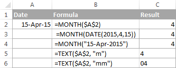
This is the most obvious and easiest way to convert date to month in Excel. For example:
=MONTH(A2)- returns the month of a date in cell A2.=MONTH(DATE(2015,4,15))- returns 4 corresponding to April.=MONTH("15-Apr-2015")- obviously, returns number 4 too.
TEXT function in Excel - extract month as a text string
An alternative way to get a month number from an Excel date is using the TEXT function:
=TEXT(A2, "m")- returns a month number without a leading zero, as 1 - 12.=TEXT(A2,"mm")- returns a month number with a leading zero, as 01 - 12.
Please be very careful when using TEXT formulas, because they always return month numbers as text strings. So, if you plan to perform some further calculations or use the returned numbers in other formulas, you'd better stick with the Excel MONTH function.
The following screenshot demonstrates the results returned by all of the above formulas. Please notice the right alignment of numbers returned by the MONTH function (cells C2 and C3) as opposed to left-aligned text values returned by the TEXT functions (cells C4 and C5).
How to extract month name from date in Excel
In case you want to get a month name rather than a number, you use the TEXT function again, but with a different date code:
=TEXT(A2, "mmm")- returns an abbreviated month name, as Jan - Dec.=TEXT(A2,"mmmm")- returns a full month name, as January - December.

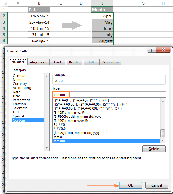
If you don't actually want to convert date to month in your Excel worksheet, you are just wish to display a month name only instead of the full date, then you don't want any formulas.
Select a cell(s) with dates, press Ctrl+1 to opent the Format Cells dialog. On the Number tab, select Custom and type either "mmm" or "mmmm" in the Type box to display abbreviated or full month names, respectively. In this case, your entries will remain fully functional Excel dates that you can use in calculations and other formulas. For more details about changing the date format, please see Creating a custom date format in Excel.
How to convert month number to month name in Excel
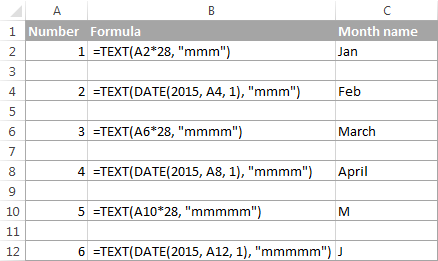
Suppose, you have a list of numbers (1 through 12) in your Excel worksheet that you want to convert to month names. To do this, you can use any of the following formulas:
To return an abbreviated month name (Jan - Dec):
=TEXT(A2*28, "mmm")
=TEXT(DATE(2015, A2, 1), "mmm")
To return a full month name (January - December):
=TEXT(A2*28, "mmmm")
=TEXT(DATE(2015, A2, 1), "mmmm")
In all of the above formulas, A2 is a cell with a month number. And the only real difference between the formulas is the month codes:
- "mmm" - 3-letter abbreviation of the month, such as Jan - Dec
- "mmmm" - month spelled out completely
- "mmmmm" - the first letter of the month name
How these formulas work
When used together with month format codes such as "mmm" and "mmmm", Excel considers the number 1 as Day 1 in January 1900. Multiplying 1, 2, 3 etc. by 28, you are getting Days 28, 56, 84, etc. of the year 1900, which are in January, February, March, etc. The format code "mmm" or "mmmm" displays only the month name.
How to convert month name to number in Excel
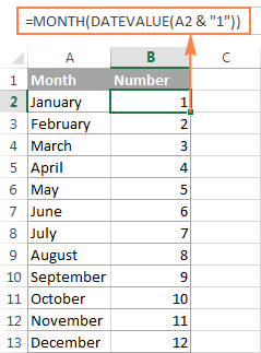
There are two Excel functions that can help you convert month names to numbers - DATEVALUE and MONTH. Excel's DATEVALUE function converts a date stored as text to a serial number that Microsoft Excel recognizes as a date. And then, the MONTH function extracts a month number from that date.
The complete formula is as follows:
=MONTH(DATEVALUE(A2 & "1"))
Where A2 in a cell containing the month name you want to turn into a number (&"1" is added for the DATEVALUE function to understand it's a date).
How to get the last day of month in Excel (EOMONTH function)
The EOMONTH function in Excel is used to return the last day of the month based on the specified start date. It has the following arguments, both of which are required:
- Start_date - the starting date or a reference to a cell with the start date.
- Months - the number of months before or after the start date. Use a positive value for future dates and negative value for past dates.
Here are a few EOMONTH formula examples:
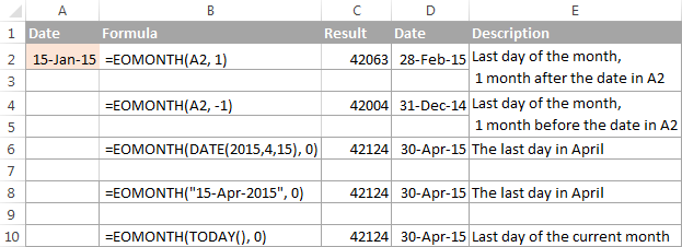
=EOMONTH(A2, 1) - returns the last day of the month, one month after the date in cell A2.
=EOMONTH(A2, -1) - returns the last day of the month, one month before the date in cell A2.
Instead of a cell reference, you can hardcode a date in your EOMONTH formula. For example, both of the below formulas return the last day in April.
=EOMONTH("15-Apr-2015", 0)
=EOMONTH(DATE(2015,4,15), 0)
To return the last day of the current month, you use the TODAY() function in the first argument of your EOMONTH formula so that today's date is taken as the start date. And, you put 0 in the months argument because you don't want to change the month either way.
=EOMONTH(TODAY(), 0)
Note. Since the Excel EOMONTH function returns the serial number representing the date, you have to apply the date format to a cell(s) with your formulas. Please see How to change date format in Excel for the detailed steps.
And here are the results returned by the Excel EOMONTH formulas discussed above:
If you want to calculate how many days are left till the end of the current month, you simply subtract the date returned by TODAY() from the date returned by EOMONTH and apply the General format to a cell:
=EOMONTH(TODAY(), 0)-TODAY()
How to find the first day of month in Excel
As you already know, Microsoft Excel provides just one function to return the last day of the month (EOMONTH). When it comes to the first day of the month, there is more than one way to get it.
Example 1. Get the 1st day of month by the month number
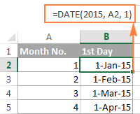
If you have the month number, then use a simple DATE formula like this:
For example, =DATE(2015, 4, 1) will return 1-Apr-15.
If your numbers are located in a certain column, say in column A, you can add a cell reference directly in the formula:
=DATE(2015, B2, 1)
Example 2. Get the 1st day of month from a date
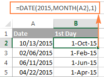
If you want to calculate the first day of the month based on a date, you can use the Excel DATE function again, but this time you will also need the MONTH function to extract the month number:
For example, the following formula will return the first day of the month based on the date in cell A2:
=DATE(2015,MONTH(A2),1)
Example 3. Find the first day of month based on the current date
When your calculations are based on today's date, use a liaison of the Excel EOMONTH and TODAY functions:
=EOMONTH(TODAY(),0) +1 - returns the 1st day of the following month.
As you remember, we already used a similar EOMONTH formula to get the last day of the current month. And now, you simply add 1 to that formula to get the first day of the next month.
In a similar manner, you can get the first day of the previous and current month:
=EOMONTH(TODAY(),-2) +1 - returns the 1st day of the previous month.
=EOMONTH(TODAY(),-1) +1 - returns the 1st day of the current month.
You could also use the Excel DATE function to handle this task, though the formulas would be a bit longer. For example, guess what the following formula does?
=DATE(YEAR(TODAY()), MONTH(TODAY()), 1)
Yep, it returns the first day of the current month.
And how do you force it to return the first day of the following or previous month? Hands down :) Just add or subtract 1 to/from the current month:
To return the first day of the following month:
=DATE(YEAR(TODAY()), MONTH(TODAY())+1, 1)
To return the first day of the previous month:
=DATE(YEAR(TODAY()), MONTH(TODAY())-1, 1)
How to calculate the number of days in a month
In Microsoft Excel, there exist a variety of functions to work with dates and times. However, it lacks a function for calculating the number of days in a given month. So, we'll need to make up for that omission with our own formulas.
Example 1. To get the number of days based on the month number
If you know the month number, the following DAY / DATE formula will return the number of days in that month:
In the above formula, the DATE function returns the first day of the following month, from which you subtract 1 to get the last day of the month you want. And then, the DAY function converts the date to a day number.
For example, the following formula returns the number of days in April (the 4th month in the year).
=DAY(DATE(2015, 4 +1, 1) -1)
Example 2. To get the number of days in a month based on date
If you don't know a month number but have any date within that month, you can use the YEAR and MONTH functions to extract the year and month number from the date. Just embed them in the DAY / DATE formula discussed in the above example, and it will tell you how many days a given month contains:
=DAY(DATE(YEAR(A2), MONTH(A2) +1, 1) -1)
Where A2 is cell with a date.
Alternatively, you can use a much simpler DAY / EOMONTH formula. As you remember, the Excel EOMONTH function returns the last day of the month, so you don't need any additional calculations:
=DAY(EOMONTH(A1, 0))
The following screenshot demonstrates the results returned by all of the formulas, and as you see they are identical:

How to sum data by month in Excel
In a large table with lots of data, you may often need to get a sum of values for a given month. And this might be a problem if the data was not entered in chronological order.
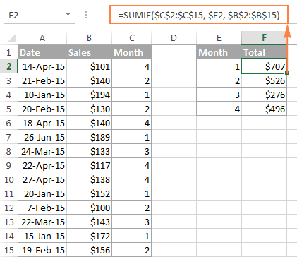
The easiest solution is to add a helper column with a simple Excel MONTH formula that will convert dates to month numbers. Say, if your dates are in column A, you use =MONTH(A2).
And now, write down a list of numbers (from 1 to 12, or only those month numbers that are of interest to you) in an empty column, and sum values for each month using a SUMIF formula similar to this:
=SUMIF(C2:C15, E2, B2:B15)
Where E2 is the month number.
The following screenshot shows the result of the calculations:
If you'd rather not add a helper column to your Excel sheet, no problem, you can do without it. A bit more trickier SUMPRODUCT function will work a treat:
=SUMPRODUCT((MONTH($A$2:$A$15)=$E2) * ($B$2:$B$15))
Where column A contains dates, column B contains the values to sum and E2 is the month number.
Note. Please keep in mind that both of the above solutions add up all values for a given month regardless of the year. So, if your Excel worksheet contains data for several years, all of it will be summed.
How to conditionally format dates based on month
Now that you know how to use the Excel MONTH and EOMONTH functions to perform various calculations in your worksheets, you may take a step further and improve the visual presentation. For this, we are going to use the capabilities of Excel conditional formatting for dates.
In addition to the examples provided in the above mentioned article, now I will show you how you can quickly highlight all cells or entire rows related to a certain month.
Example 1. Highlight dates within the current month
In the table from the previous example, suppose you want to highlight all rows with the current month dates.
First off, you extract the month numbers from dates in column A using the simplest =MONTH($A2) formula. And then, you compare those numbers with the current month returned by =MONTH(TODAY()). As a result, you have the following formula which returns TRUE if the months' numbers match, FALSE otherwise:
=MONTH($A2)=MONTH(TODAY())
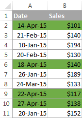
Create an Excel conditional formatting rule based on this formula, and your result may resemble the screenshot below (the article was written in April, so all April dates are highlighted).
Example 2. Highlighting dates by month and day
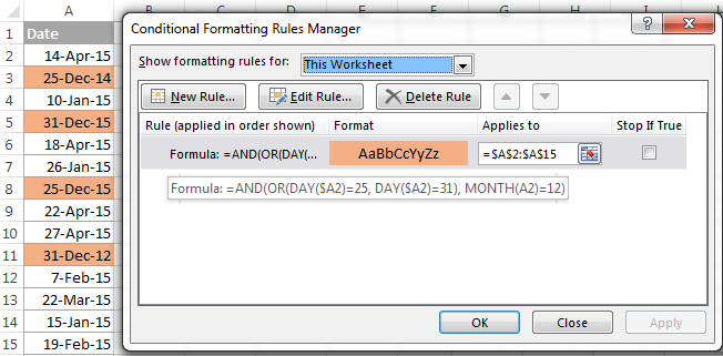
And here's another challenge. Suppose you want to highlight the major holidays in your worksheet regardless of the year. Let's say Christmas and New Year days. How would you approach this task?
Simply use the Excel DAY function to extract the day of the month (1 - 31) and the MONTH function to get the month number, and then check if the DAY is equal to either 25 or 31, and if the MONTH is equal to 12:
=AND(OR(DAY($A2)=25, DAY($A2)=31), MONTH(A2)=12)
This is how the MONTH function in Excel works. It appears to be far more versatile than it looks, huh?
In a couple of the next posts, we are going to calculate weeks and years and hopefully you will learn a few more useful tricks. If you are interested in smaller time units, please check out the previous parts of our Excel Dates series (you will find the links below). I thank you for reading and hope to see you next week!
 by
by
451 comments
Hi Alexander, you help me with if i have the number of years and months how can get the first date,month and year for that range.
Ex. if i want the calculate what the date was from 04 months from today, it should be 01-01-2021
how can i apply that into excel ? if i add year and moth on 2 different cells and it has to return the date. considering excel date as today
Hello!
I recommend reading this guide: Subtract dates in Excel; add days, weeks, months or years to date.
I want next month target to be automatically generated no matter what time of year we look at it. (target getting from table)
I need to a formula for convert different date's of Month name with year
Hello!
Please check out this article to learn how to extract month name from date.
I recommend reading this guide: Excel YEAR function - convert date to year
I hope my advice will help you solve your task.
I have expiration date and I need to find out expiration range like 0 to 3 Month or 3 to 6 Months in excel
Hi,
I recommend reading this guide:
Excel DATEDIF - calculating date difference in days, weeks, months.
If this is not what you wanted, please describe the problem in more detail.
This is the date format ( 20201101 ) which I have right now. Tell me how to get my month name in Text Eg, "Jan"
Hello!
If I got you right, the formula below will help you with your task:
=TEXT((--RIGHT(A2,2))*28, "mmm")
HI There,
I'm not incredibly advanced on excel and am having some trouble, not sure I can adequately explain my requirements.
I have a large table of information that requires 3 sets of conditional formats that will highlight the entire line if affected by certain date ranges. And I can't figure it out.
The cell I am working with is 'Shipment Period' which is based on the whole month.
I need all line data, that:
1. Falls before (past date) the current month e.g. 2021-02; to be highlighted pink/red
2. Falls during the current month; to be highlighted green
3. Falls after (future dated) the current month; to be highlighted orange
Any assistance would be appreciated.
Hello!
Please check out the following article on our blog, it’ll be sure to help you with your task: Excel conditional formatting for dates & time
I hope my advice will help you solve your task.
I need to a formula
that s will be start month from 16th and end of the next month 15th days
For example 2/16 to 3/15.
Hi,
The information you provided is not enough to understand your case and give you any advice. What source data is used for this task? The expected result is two dates or text? Please describe your problem in more detail.
How to calculate month + 3 days in excel
Hello!
If I understand your task correctly, check out this article to learn how to add days to date in Excel.
If this is not what you wanted, please describe your problem in more detail.
i want to see if cell a2 show 23.11.2020
than i want to see cell b2 show 23.12.2020 how to write formula
Dear Mam,
When we calculate no. of months for by DATEDIF function, result obtained is incorrect.
Please advise & suggest necessary formulas.
Start date-1-July-21 (A1)
End date-31-Dec-21 (A2)
Formula =DATEDIF(A1,A2,"M")
Result from function=5
Correct result=6
Thanks
I just want to know how to change my date to April 1st
Hello!
Specify which date you want to change.
Pay attention to this comment.
Hello
I have a series of dates in column B and a series of numbers in column L. I want to add the numbers when the month is October. I thought of
=SUMIF(B2:B89,"MONTH=10",L2:L89)
but it gives 0. What is the way to do it.
Thank you
Hello!
Use SUMPRODUCT function. The formula below will do the trick for you:
=SUMPRODUCT($L$2:$L$89,--(MONTH($B$2:$B$89)=10))
Hope this is what you need.
Yes thank you that worked
Hi.
what function to used for converting 15-Oct-20 to Oct'20?
Hello!
You can use custom date format
mmm"'"yy
Hope this is what you need.
hi
i have numbers in a columnlike 1,2,6,7,,4,657,4986,343,113,4245, in another column i want a oformula whichh will find the result of number of months against the days
Hello!
I’m sorry but your task is not entirely clear to me. Could you please describe it in more detail? How are these numbers and dates related? What result do you want to get? Give an example of the source data and the expected result.
Dear sirs, can I ask for a wee bit of your expertise since my own is not enough in this case?
I am looking to do comparisons between quarters during the year but with the closing balance date fixed from previous year. Let me explain:
E.g. QUARTER 4(b)=2020-12-31, QUARTER 3(c)=2020-09-30, Closing balance (QUARTER 4(a))=2019-12-31.
I have created formulas for Q4(b) and Q3(c) (linked to another date cell with the help of your EOMONTH-functions on this page) respecively so that when Q4(b)=>Q1(b), Q3(c)=>Q4(c). But, i want the Closing balance date Q4(a) (ie. 2019-12-31) to remain the same during the year UNTILL the new accounting year starts. So when Q1(b)=2021-03-31, Q4(c)=2020-12-31 and Q4(a)=2020-12-31.
In words, Q(b) and Q(c) change during the year where Q(a) remain the same with previous year's closing date, and it's only when the Q(b)/Q(c) year change as Q(a) changes closing date one year forward.
I find the Q(a) value quite tricky to solve.
Thank you and regards,
Daniel
There are different dates in excel in each cell. if date is 1st of any month then that should be changed to last date of previous month and if date is 2nd or any other from 2 to 31 then the date should change to last date of that month.
please help with formula in excel
Hello!
If I understand your task correctly, the following formula should work for you:
=IF(DAY(A1)>1,EOMONTH(A1,0),EOMONTH(A1,-1))
I hope my advice will help you solve your task.
Hello,
May I know how to extract the last day of the month if there is only year and month mentioned in general format? For example, 2020-06? The answer I am looking for is 06/30/2020?
Thanks,
Prashant S
Hello!
If I understand your task correctly, the following formula should work for you:
=EOMONTH(B1,0)
Hope this is what you need.
Hi,
I am trying to calculate and convert the current month to "currentmonth" using today date and month.
01/04/2020, 10:15:00
how to convert this in to month
Hello!
I hope you have studied the recommendations in the tutorial above.
i have tried but i can't get the result, can you please give me the formula which will help me to get month when it appears in this format. 01/04/2020, 10:15:00
Hello!
You did not say anything about this, but I can assume that your date is recorded as text. Therefore, you need to remove the comma from it and convert it to a date. And then apply the MONTH function:
=MONTH(DATEVALUE(SUBSTITUTE(D1,",","")))
I hope this will help
Thanks,
So, there is no option without removing , in this format.
Hi,
I need your help.
Column A = Completion of project (Date format: 01-Jul-2020)
Column B = Invoicing Month (Month format: July 2020)
Items completed within 1st - 25th of every month must be invoiced in that month itself and items completed from 26th-31st is to be invoiced the next month.
Any ideas how I can set a rule so Column B is generated based on the dates automatically?
Hello Sammy!
The formula below will do the trick for you:
=IF(DAY(A1)<26,A1,EOMONTH(A1,0)+1)
Remember to set the date format in cell B correctly
Correction: Martch duration = 22 days, April duration = 22 days, May duration = 11 days. Thanks.
Hi Alexander,
I have data as below:
Task start_day end_day duration, d
Task1 01/03/2020 15/05/2020 55
I have to show task duration by month in the chart. How can I get data needed for chart? I need: Martch duration = 20 days, April duration = 20 days, May duration = 15 days. Thanks.
Hello Ruta!
I’m sorry but your task is not entirely clear to me.
Please describe your problem in more detail. Include an example of the source data and the result you want to get. It’ll help me understand your request better and find a solution for you. Thank you.
Sry I forgot to add the formula I'm using. =SUMIF(O6:O24, AN6, AJ6:AJ24)
Hello,
I have used the formula above and only changed the cells, however the result sum to $0. Do the cells need to be together to work because these are not.
Thankyou
Hello Mark!
The formula is spelled correctly. But you asked your question in the wrong article. I recommend that you study this instruction about the SUMIF function.
in case if you got 00 your computer's language setup is the problem
use this: =TEXT(A1;"[$-en-EN]HHHH")
en-EN ---> add here the language's code you want to see
HHHH ---> the version of MMMM (month full lenght) in your computer's language
Your version can be checked in Format Cells - Custom ---> last two options
I am doing a monthly billing spreadsheet where I have listed income by each month, this is along side the bill,amount, and due date. At the bottom I am wanting the extra money left from each month calculation, needing it to register which month it is and bring that months income amount - the current months bills. Example below.
Due Date Bills Amount Month Wks Income(mthly)
7th Car $365 January 4 $2000
8th Netflix $13 February 4 $2000
Total Monthly Expenses $478 Leftover ____?????_____
Hello LeAnn !
I’m sorry but your task is not entirely clear to me. For me to be able to help you better, please describe your task in more detail. Please specify what you were trying to find, what formula you used and what problem or error occurred.How is 478 calculated? Give more an example of the source data and the expected result.
It’ll help me understand it better and find a solution for you. Thank you.
hello. i have a question and it may be stupid if this doesn't exist in excel. :D
is there a command/formula to change all the written month (ex: January) and change it to the next month (ex: February) rather than changing/typing it one by one. i wanted to make the changes faster since the 2 sheet file will be used for the entire year except the months have to be changed.
thank you for your time. :)
I need a format for if a date has is in the last month to return another cell and if its not in the past month to return blank
Hello Ben!
Using cell formatting, your problem cannot be solved. If you need a formula, describe in more detail all the conditions. Please describe your problem in more detail. It’ll help me understand it better and find a solution for you. Thank you.
I am a registered dog breeder and I would like to create in excel a schedule for the litter. I cannot breed two litters in 18 months. How do input my last litter so when I look at it when the right month and year to breed her. I only have 3 dogs.if it's under this month, to show in red. Anyone can help?
Hello!
I’m sorry but your task is not entirely clear to me. You need to use conditional formatting. What data do you use in the table?
For me to be able to help you better, please describe your task in more detail. It’ll help me understand it better and find a solution for you. Thank you.
Currently using this [WEEKNUM(TODAY(), 1)-WEEKNUM(DATE(YEAR(TODAY()), MONTH(TODAY()), 1), 1)+1)] in a countif formula. However what would would i do if i wanted to have a month to date look. Ex Week 1 would just be week 1. and week 2 it would be week one + week two and so on.
Hello!
Your formula calculates the week number in the current month. But I don’t understand what else do you want to calculate? Explain in more detail so that I can help you.
Hi alexander,
Correct. Its currently calculating to look at the current week. IN my scenario I have bunch of dates all throughout the Month. And depending on the week i am in, i calculate how many of those dates fall within the same week that were are in. What i am wanting to do is to adjust that to give me a running total. For example, if i was in week 2 the current formula will just looks at all the dates that are in the second week and count those. Instead I'm wondering if we could alter the formula to look at all the past weeks of the month as well. So if we are in week 2, the formula would Look at week 2 + week 1. I hope i was able to clarify this.
Hello
If I understand your task correctly , if the date is written in cell C1, and the formula
= WEEKNUM (C1,1) -WEEKNUM (DATE (YEAR (C1), MONTH (C1), 1), 1) +1
in cell D1,
then the condition for the counter of the desired dates
= COUNTIFS($D$1:$D$99, D1) + COUNTIFS($D$1:$D$99, D1-1)
I hope this will help, otherwise please do not hesitate to contact me anytime.
Hi Alexander,
I want to know the formula to get the particular day of every month in the given data.
Hello Vaibhav!
I think you need to read an article on our blog about calculating days of the week in Excel.
Hi Alexander
This was very helpful for my first part of the task. I have now taken the month from a date and shown it as the Month in text. I now want to take that result and have it sequence monthly for 24 months across a row, but I am having trouble reference that result and indexing it across the columns. Can you advise?
I am a beginner in Excel, so trying to learn what I can as I need it.
Thank you!
Hello Glenn!
If I understand your task correctly, in cell A1 is your start date. In cell A2, write the formula
=TEXT(EDATE($A$1,COLUMN()-1), "mmmm")
After that you can copy this formula right along the row.
If there is anything else I can help you with, please let me know.
By using countif() I derive the total number of records of each branch as usual I want data regards specific month
Hello Madhavi!
Use the expression as a condition: MONTH(D1)=4 where D1 is the date cell.
For me to be able to help you better, please describe your task in more detail. It’ll help me understand it better and find a solution for you. Thank you.
I use a spreadsheet for monthly budget reports. Each month has a YTD column. The formula typically looks like this: ='[March 2019]MARCH 2019'!E3+'APRIL 2019'!B3
In this example, April is added to March's YTD totals in that column. When setting up the sheet for 2020, I have been unable to get it to change the whole column of totals. It will only change one cell at a time although I have included all cells.
Hello Gojo!
Unfortunately, you have not written what you managed to change in your formula and what you did not manage to change. It is not clear enough what exactly is not working.
Perhaps, there is a problem with the names of the files in your formula, but it is merely my assumption.
Please describe your problem in more detail and I will try to help you.
I have downloaded a data which is from Jan-2020 to mar 2020, like below:
05/02/2020 06:09 - It is showing month as May
1/31/2020 2:55 AM - This one is showing Jan
1/29/2020 12:27 AM
1/17/2020 6:47 AM
1/16/2020 5:39 AM
1/14/2020 7:46 AM
06/01/2020 03:41 - This one showing as June 20202.
I tried converting it into month through text formula, tried changing format through data tab to convert text to column, also manually tried custom formatting but no go.
Please help me in rectifying this.
Hello Himanshu!
Please go to Format Cells, choose Number -> Custom Format and set
mmm-yyyy;@
to display the date as Jan 2020,
mmmm;@
to display the date as January.
I hope you will find my advice helpful.
I need to take a date from this format 3/31/2020 to the "31st day of March 2020". I have NO problem on the March 2020 part but HOW in the world can I get the st part of 31st ??? Also need the abbreviations for all days 1, 2, 3, ..... 29, 30, and 31. Like 1st. 2nd, 3rd, and so on. The Only workaround I can think of is to create a table or chart with all the possible numbers with abbreviations and then use vlookup or the new xlookup.
Thanks in advance for any help or insight !!!
Hello Carl!
If I understand your task correctly, the following formula convert to ordinal date format:
=DAY(A1)&IF(OR(DAY(A1) = {1,2,3,21,22,23,31}),CHOOSE (1*RIGHT(DAY(A1),1),"st ","nd ","rd "),"th")&TEXT(A1,"mmmm, yyyy")
or
=DAY(A1)&IF(OR(DAY(A1) = {1,2,3,21,22,23,31}),CHOOSE (1*RIGHT(DAY(A1),1),"st day of ","nd day of ","rd day of "),"th day of ")&TEXT(A1,"mmmm, yyyy")
I hope it’ll be helpful.
Hello Michael!
Please use the following formula
=DATE(YEAR(A1)+2, MONTH(A1)+9, DAY(A1)+0) or
=DATE(YEAR(TODAY())+2, MONTH(TODAY())+9, DAY(TODAY())+0)
We have a ready-made solution for your task. I'd recommend you to have a look at our Ablebits Tools - Date&Time Wizard.
This tool is available as a part of our Ultimate Suite for Excel that you can install in a trial mode and use for 30 days for free: https://www.ablebits.com/files/get.php?addin=xl-suite&f=free-trial
Hello,
I have calculated the number of year and months in excel. Now I am trying to get Excel to tell me what month and year that will be from now. For example, my car note will be paid off 2 years and 9 months from now, March 29, 2020. How can I get excel to tell me that 2 years and 9 months from now will be in December 2022? I thank you for your help with respect to resolving this issue in advance.
I need a formal that if a month has 31 days it will displace from cell D5 and if then displace from cell D4. the month is in A1. Can you help me, please?
Hello, Brenda!
If I understand your task correctly, the following formula should work for you:
=IF(DAY (EOMONTH (DATE(2020,A1,1),0)) = 31, D5, D4)
Thanks a lot for your information. I have an issue to convert the following text date to a real date type.
Jan 02, 2018
Would you help on how I can convert it to date type? I've tried "=date(RIGHT(A2,4) LEFT(A2,3) MID(A2,5,2))", but it doesn't work.
Hello? Mark!
Please use the following formula
=DATEVALUE(A2)
=DATA.VALue(replace(replace(a2;".";"/");" de ";""))
01/01/2020 AMUH
02/01 DLD
03/01 AMUH
04/01 ARASH
05/01 DAFZA
02/02/2020 AMUH
04/02/2020 UTPM
01/03/2020 UPTM
07/03/2020 AMUH
04/04/2020 AMUH
HOW CAN WE CALCULATE MONT WISE
KINDLY SHOW THE CALCULATION
I have few date range with different months and year. I want to hight only date which are from January to June regardless year. Can you please help me for this?
Example.
04-12-2006
05-06-2007
20-08-2008
05-01-2009
09-11-2007
25-06-2008
08-01-2009
24-06-2008
01-02-2011
17-11-2011
24-09-2011
05-09-2012
30-09-2011
24-09-2011
04-07-2019
04-01-2009
31-12-2013
01-12-2013
01-12-2013
01-12-2013
22-01-2014
25-06-2008
01-12-2013
17-02-2012
01-12-2013
12-03-2016
12-03-2016
12-03-2016
12-03-2016
12-03-2016
12-12-2017
07-05-2019
10-07-2019
10-06-2019
05-07-2019
05-07-2019
29-07-2019
28-09-2019
from above dates I want to hightligh only dates from January to June regardless year.
Hi,
Struggled to understand this, =TEXT(A2*28, "mmmm"). Why multiply by 28?
Hi Sam,
Thank you for a very good question!
In its internal system, Excel considers the number 1 as Day 1 in January 1900 (when used together with month format codes such as "mmm" and "mmmm"). By multiplying the numbers 1, 2, 3 etc. by 28, you are getting Days 28, 56, 84, etc. which are in January, February, March, etc. Multiplying by 29 will also work.
I've also added this explanation to the tutorial for other readers.
I am facing a problem that I am using to display a stacked bar chart with "Time" as the timeline. However, I don't know how to make the x-axis (timeline) to display 1st day of each month. Any idea?
hi
i have one question, i have the calendar in excel and i am entering holidays next to the particular date. when i change the month, how i can clear the my holiday entries automatically.
thanks
Problem solved:
I used this-
=AND(MONTH($A1)=MONTH(TODAY()),YEAR($A1)=YEAR(TODAY()))
Problem solved:
I used this-
=AND(MONTH($A1)=MONTH(TODAY()),YEAR($A1)=YEAR(TODAY()))
Now I want the rest of the date should be highlighted in yellow colour. I mean if the month and the year is less than or more than today's month and the year it should be highlighted in yellow colour.
I have different dates in column A1 (1-Oct-19, 15-Oct-19,29-Oct-19, 12-Nov-19, 26-Nov-19, 10-Jan-21 and so on). I want to highlight only the current month in green and the rest of the month in the red. I mean before and after Jan in the red and Jan (Current Month) in green.
Example 1. Highlight dates within the current month
=MONTH($A2)=MONTH(TODAY())
Through this, if year changes it is highlighting the same month also. How can I highlight the date within the current month and year?
10-Jan-20, 15-Jan-21
It will highlight both cells. When the year is 2020, it should not highlight the year 2021.
I have dates in a row (dates span across months) and certain values in the cells below these dates (e.g. work shifts such as "M" for morning). I need to count number of occurrences of a shift per month. How to I achieve this ?
I tried using MONTH() and COUNTIF()/COUNTIFS() together but failed.
if i have a sum or number like 28, 30 or 31 how i count these no. as 1 month
i try formula =DATEDIF(0,F26,"ym") but it show 0 and formula =DATEDIF(0,F26,"md") it show same no. as 28, 30 & 31.
i want it show as 1 month if any solution or formula pls.
how calculate the sum 31 as a month or how to show 31 as (1 month or 1) in excel
i try =DATEDIF(0,F25,"ym") (where F25 is a no. or sum =31) but is show only 31 as result instead of 1.