The tutorial shows how to extract number from various text strings in Excel by using formulas and the Extract tool.
When it comes to extracting part of a text string of a given length, Excel provides three Substring functions (Left, Right and Mid) to quickly handle the task. When it comes to extracting numbers from an alphanumeric string, Microsoft Excel provides… nothing.
To get a number from a string in Excel, it takes a little ingenuity, a bit of patience, and a bunch of different functions nested into each other. Or, you can run the Extract tool and have the job done with a mouse click. Below you will find full details on both methods.
How to extract number from the end of text string
When you have a column of alphanumeric strings where number comes after text, you can use the following formula to get it.
We will dwell on the formula's logic a bit later. For now, simply replace cell with a reference to the cell containing the original string (A2 in our case), and enter the formula in any empty cell in the same row, say in B2:
=RIGHT(A2, LEN(A2) - MAX(IF(ISNUMBER(MID(A2, ROW(INDIRECT("1:"&LEN(A2))), 1) *1)=FALSE, ROW(INDIRECT("1:"&LEN(A2))), 0)))
This formula gets number only from the end. If a string also has numbers in the beginning or middle, they are ignored:
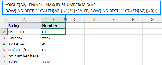
The extraction is performed with the RIGHT function that belongs to the category of Text functions. The output of this function is always text. In our case, the result is a numeric substring, which in terms of Excel is also text, not number.
If you need the result to be a number (that you can use in further calculations), then wrap the formula into the VALUE function or perform an arithmetic operation that does not change the result, say, multiply by 1 or add 0. To catch errors in the strings that do not contain a single number, use the IFERROR function. For example:
=IFERROR(VALUE(RIGHT(A2, LEN(A2) - MAX(IF(ISNUMBER(MID(A2, ROW(INDIRECT("1:"&LEN(A2))), 1)*1)=FALSE, ROW(INDIRECT("1:"&LEN(A2))), 0)))), "")
or
=IFERROR(RIGHT(A2, LEN(A2) - MAX(IF(ISNUMBER(MID(A2, ROW(INDIRECT("1:"&LEN(A2))), 1) *1)=FALSE, ROW(INDIRECT("1:"&LEN(A2))), 0))) +0, "")
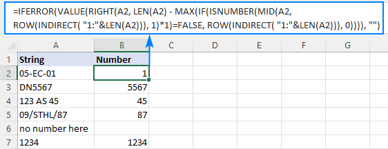
Note. In Dynamic Array Excel (Office 365 and 2021), you enter the formula in the usual way with the Enter key. In Excel 2019 and earlier, it only works as an array formula, so remember to press Ctrl + Shift + Enter to complete it.
How this formula works:
To extract number from an alphanumeric string, the first thing you need to know is where to start the extraction. The position of the last non-numeric character in a string is determined with the help of this tricky formula:
MAX(IF(ISNUMBER(MID(A2, ROW(INDIRECT("1:"&LEN(A2))), 1)*1)=FALSE, ROW(INDIRECT("1:"&LEN(A2))), 0))
To understand the logic, let's investigate it from the inside:
The ROW(INDIRECT("1:"&LEN(A2))) combination creates a sequence of numbers corresponding to the total of characters in the source string (A2), and we serve these sequential numbers to MID as the starting numbers:
MID(A2, {1;2;3;4;5;6;7;8}, 1)
The MID function pulls each individual character from A2 and returns them as an array:
{"0";"5";"-";"E";"C";"-";"0";"1"}
As MID is a text function, its output is always text (as you can notice, all the characters are enclosed in quotation marks). To turn numeric ones into numbers, we multiply the array by 1 (double negation --MID() will have the same effect). The result of this operation is an array of numbers and #VALUE! errors representing non-numeric characters:
ISNUMBER({0;5;#VALUE!;#VALUE!;#VALUE!;#VALUE!;0;1})
The ISNUMBER function evaluates each element of the array and gives its verdict in the form of Boolean values - TRUE for numbers, FALSE for anything else:
{TRUE;TRUE;FALSE;FALSE;FALSE;FALSE;TRUE;TRUE}
This array goes to the logical test of the IF function, where each element of the array is compared against FALSE:
IF({TRUE;TRUE;FALSE;FALSE;FALSE;FALSE;TRUE;TRUE}=FALSE, ROW(INDIRECT("1:"&LEN(A2))), 0)
For each FALSE (non-numeric value), another ROW(INDIRECT()) function returns its relative position in the string. For each TRUE (numeric value), a zero is returned. The resulting array looks as follows:
{0;0;3;4;5;6;0;0}
The rest is easy. The MAX function finds the highest number in the above array, which is the position of the last non-numeric value in the string (6 in our case). Simply, subtract that position from the total length of the string returned by LEN, and pass the result to RIGHT to let it know how many characters to extract from the right side of the string:
RIGHT(A2, LEN(A2) - 6)
Done!
How to extract number from the beginning of text string
If you are working with records where text appears after number, you can extract number from the start of a string by using this generic formula:
With the original string in A2, use the following formula to get number:
=LEFT(A2, MATCH(FALSE, ISNUMBER(MID(A2, ROW(INDIRECT("1:"&LEN(A2)+1)), 1) *1), 0) -1)
No matter how many digits are in the middle or end, only the starting number is extracted:

Note. In Excel 365 and Excel 2021, due to support for dynamic arrays, a regular formula works fine. In Excel 2019 and earlier, you should press Ctrl + Shift + Enter to explicitly make it an array formula.
How this formula works:
Here, we again use the combination of ROW, INDIRECT and LEN functions to create a sequence of numbers equal to the total of characters in the source string plus 1 (the role of that additional character will become clear a bit later).
ROW(INDIRECT("1:"&LEN(A2)+1))
MID and ISNUMBER do the same job as in the previous example - MID pulls individual characters and ISNUMBER converts them to the logical values. The resulting array of TRUE's and FALSE's goes to the MATCH function as a lookup array:
MATCH(FALSE, {TRUE;TRUE;FALSE;FALSE;FALSE;FALSE;TRUE;TRUE;FALSE}, 0)
MATCH computes a relative position of the first FALSE, giving us the position of the first non-numeric character in the string (3 in A2). To extract the preceding numbers, we subtract 1 from position the first text character and serve the difference to the num_chars argument of the LEFT function:
LEFT(A2, 3-1)
Now, back to an "extra" character in the sequence generated by ROW(INDIRECT()+1)). As you already know, this sequence provides the starting points for the MID function. Without +1, MID would extract exactly as many characters as there are in the original string. If the string contains only numbers, ISNUMBER will return only TRUE's while MATCH needs at least one FALSE. To ensure that, we add one more character to the total length of the string, which the MID function would convert to an empty string. For example, in B7, MID returns this array:
{"1";"2";"3";"4";""}
Note. As is the case with the RIGHT function, LEFT also returns a numeric substring, which is technically text, not number. To get the result as a number rather than a numeric string, nest the formula in the VALUE function or multiply the result by 1 as shown in the first example.
How to get number from any position in a string
If your task implies extracting number from anywhere in a string, you can make use of the following mind-boggling formula published on MrExcel forum:
=SUMPRODUCT(MID(0&A2, LARGE(INDEX(ISNUMBER(--MID(A2, ROW(INDIRECT("1:"&LEN(A2))), 1)) * ROW(INDIRECT("1:"&LEN(A2))), 0), ROW(INDIRECT("1:"&LEN(A2))))+1, 1) * 10^ROW(INDIRECT("1:"&LEN(A2)))/10)
Where A2 is the original text string.
Breaking down this formula would require a separate article, so you can simply copy it to your worksheet to make sure it really works :)
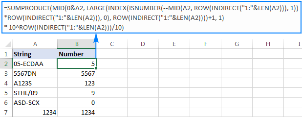
Upon examining the results, however, you may notice one insignificant drawback - if the source string does not contain a number, the formula returns zero, as in row 6 in the screenshot above. To fix this, you can wrap the formula in the IF statement, the logical test of which checks if the source string contains any number. If it does, the formula extracts the number, otherwise returns an empty string:
=IF(SUM(LEN(A2)-LEN(SUBSTITUTE(A2, {"0","1","2","3","4","5","6","7","8","9"}, "")))>0, SUMPRODUCT(MID(0&A2, LARGE(INDEX(ISNUMBER(--MID(A2,ROW(INDIRECT("$1:$"&LEN(A2))),1))* ROW(INDIRECT("$1:$"&LEN(A2))),0), ROW(INDIRECT("$1:$"&LEN(A2))))+1,1) * 10^ROW(INDIRECT("$1:$"&LEN(A2)))/10),"")
As shown in the screenshot below, the improved formula works beautifully (kudos to Alex, our Excel guru, for this improvement):
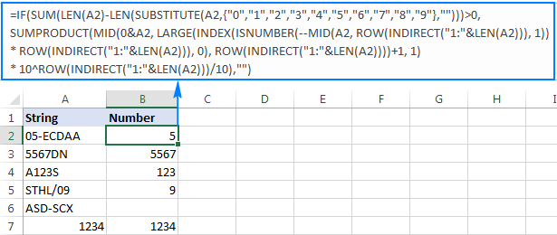
Unlike in all previous examples, the result of this formula is number. To make sure of this, just notice the right-aligned values in column B and truncated leading zeros.
Tip. In Excel 365 - Excel 2019, there is a much simpler solution with the help of the TEXTJOIN function. Please see How to remove text and keep numbers.
Extract number from text string with Ultimate Suite
As you have just seen, there is no trivial Excel formula to pull number from a text string. If you have difficulties with understanding the formulas or tweaking them for your data sets, you may like this simple way to get number from string in Excel.
With our Ultimate Suite added to your Excel ribbon, this is how you can quickly retrieve number from any alphanumeric string:
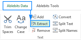
- Go to the Ablebits Data tab > Text group, and click Extract:
- Select all cells with the source strings.
- On the Extract tool's pane, select the Extract numbers radio button.
- Depending on whether you want the results to be formulas or values, select the Insert as formula box or leave it unselected (default).
My advice is to select this box if you want the extracted numbers to update automatically as soon as any changes are made to the source strings. If you want the results to be independent on the original strings (e.g. in case you plan to remove the source data at a later point), then do not select this box.
- Click the Insert Results button. Done!
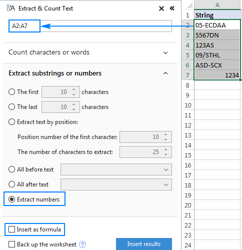
Like in the previous example, the results of the extraction are numbers, meaning you are free to count, sum, average, or perform any other calculations with them.
In this example, we've chosen to insert the results as values, and the add-in did exactly what was asked for:
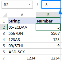
If the Insert as formula checkbox was selected, you'd observe a formula in the formula bar. Curious to know which one? Just download Ultimate Suite's trial and see for yourself :)
Available downloads
Excel Extract Number - sample workbook (.xlsx file)
Ultimate Suite - trial version (.exe file)
 by
by
546 comments
It's great! but shamelessly the formulas in english doesn't work in german... So, thanks anyway! :D
Please Help!
I have a text string containing comma delimited numbers in a single cell, e.g. "2, 3, 4, 10, 11". I am looking for a formula that looks for a given number and returns TRUE if it is contained in the string or FALSE if it is not. The formula must not confuse numbers with characters, e.g. looking for "1" in the example string above must return FALSE.
Any help much appreciated!
Type of Issue: Booking failure (order in entered status)
Here as detailed description of issue as possible.: Order 787895 is stucked can you book that. Thank you!
Order number: 787895
Priority: High
Provsiioning bars are in N/A status. Plea
----- Please help me to write excel formulate to get order numbers
Hi!
I am having trouble with my formula, despite following the instructions step by step!
I want to add numbers associated with different words. Example:
15 walk
60 gym
10 run
10 walk
30 run
I want the sum... Walk= 25 Gym=60 Run=40
To rephrase, I want the sum of all digits associated with "walk" OR "gym" OR "run".
I can't figure this one out! Thank you for any help you're able to provide!
-Stephanie
Stephanie:
Enter "Run", "Walk" and "Gym" in cells C62, D62 and E62 respectively. These will be the headers.
Enter the data in A48:A57. The formula is case sensitive so be sure the data matches the caps in the headers.
In C63 enter =SUM(IF(ISNUMBER(FIND(C62,$A$48:$A$57)),VALUE(LEFT($A$48:$A$57,FIND(C62,$A$48:$A$57)-1)),0))
then with the cursor in the formula bar in the formula click the CTRL Shift Enter keys at the same time. This is an array formula so you need to tell Excel to evaluate it as an array. When you enter the formula and then in the formula bar you put the cursor in the formula and click the CTL SHIFT ENTER keys it will put curly brackets around the formula which indicates to Excel that this is an array.
When the value appears in E63 copy the formula over to D63 and E63.
As you enter more data in the A range be sure to change the second cell address to match the last cell in the range. Right now the range is A48 to A57. If you add more data change the A57 to another cell address. Remember, there are three places in the formula for that range.
Stephanie:
I should have written:
"When the value appears in C63 copy the formula over to D63 and E63."
Hiren:
Because each of the substrings you want to are different and the strings vary in length, I think the best you can do is to use different formulas for each.
For example, with the string "XYZ 50MG TABLET" you want the "50MG" substring. You can use =MID(H35,SEARCH("MG",H35)-2,5). With the "PARADICLO 500/100MG TABLET" you can use =MID(I35,SEARCH("MG",I35)-7,9) to extract "500/100MG". This approach can be repeated for each string and substring. It's a little klunky, but I don't see anything other than the "MG" that's common to the strings.
Hi Doug,
Thanks for your response. Yes, you are right. I had already tried this and helped me in few cases. I think, for rest of the things, I will have to do manually as the description of products are different.
Once again Thanks.
Regards,
HIren
Hello,
Please help me in following.
I have a bunch of data containing product name with its strength in "MG", Like XYZ 50MG TABLET, PARADICLO 500/100MG TABLET, ABC 100 MG CAPSULE like wise....
I just need to extract "STRENGTH" like, 50MG, 500/100MG, 100MG, 0.375/0.5MG likewise.
Please help, if anyone knows.
Hiren
9898132180
Hi, I need help in extracting numbers from a string but along with spaces after each set, for ex:
A1 = first number48832234//second number552437548
Result = 48832234 552437548
i am already aware of the formula to extract all numbers.
any help is highly appreciated.
I am awaiting some help ... is someone there who can help ....
Nadeem:
I remember this question from the other day and it isn't clear. However, if you have two numbers in one cell separated by "//" and you want to remove the "//" and substitute a space then this works:
=SUBSTITUTE(A1, "//", " ")
Hi,
I am attempting to return only those numbers below which contain "50097" in the first part (before the hyphen) which are pre-fixed by "BA". The numbers need to be returned in the same cell.
BA50097-52201 BA50097-63623 BA50097-64930 BA52201-50097 BA56510-50097 BA63623-50097 BA64930-50097
I've been racking my brains. Any help would be appreciated.
Thanks,
Andrew
For clarity, I am attempting to return the second part of the string (after the hyphen) if 50097 is a match in the first part. Hope this makes sense.
I want to extract 541 from KA54115259.
Hi Jessica,
If you just need to extract 3 characters beginning with the 3rd one, you can use this formula:
=MID(A1,3,3)
Where A1 is the cell containing the original string.
Jessica,
you can use MID function in excel. It returns a specific number of characters from a text string starting at the position you specify.
in you case KA54115259 is the text string. To extract 541 from this string use =+MID(cell number,3,3). cell number in the cell where your this data appears.3 is the place of a text from where excel starts and next 3 is total number of characters you need to extract 541 i.e. 3
Can anyone help with a formula for this text string? We need the most recent date from the string. Thanks you in advanced.
Below are a few examples:
CPG PW REV 09-01-2011~No=02-19-2010~Yes=06-01-2005~Business Closing
CPG PW REV 09-29-2010
CPG PW REV 05-11-2012~No=06-08-2012~New Owner~Yes=07-21-2005~Business Closing
How do I extract the $ value?
$0.00 copayment
Rosa:
Enter this as an array formula in an empty cell and then format that cell as Number. Where the data is in C36:
=1*MID(C36,MATCH(TRUE,ISNUMBER(1*MID(C36,ROW($1:$1000),1)),0),COUNT(1*MID(C36,ROW($1:$1000),1)))
Remember, this is an array formula so after you enter it in the formula bar click in the formula and CTRL+Shift+Enter all in one click. Then you'll see the curly brackets around the entire formula indicating Excel knows this is an array formula.
Rosa:
Here's another formula to extract numbers from a string. It's also an array so CTL+Shift+Enter. I think this one works more reliably. So, where the data is in C37
=LOOKUP(10^99,--MID("|"&C37,SMALL(IF(((--ISNUMBER(--MID("|"&C37, ROW($1:$1003),1))=0)*ISNUMBER(--MID("|"&C37,ROW($2:$1004),1))),ROW($2:$1004)),1), ROW($1:$1003)))
Remember to format the cell where this formula is entered.
367 cd 046 104101 Real
131 DPU3005 104017 KRISPY
CC MERCH ID 9189997141
CC MERCH ID 9189997158
POS MID 5930005 - 06/29/2
POS MID 19520212 - 06/29/2
i want to extract 104101, 104017, 9189997141, 9189997158, 5930005, 19520212. what formula can i use to extract this numbers.
Thank you.
Hi please help me in extracting only the numbers here:
a.367 cd 046 104101 104101
b.131 DPU3005 KRISPY 104017 104017
c.CC MERCH ID 9189997141 9189997141
d.CC MERCH ID 9189997158 9189997158
e.POS MID 5930005 - 06/29/2 5930005
f.POS MID 19520212 - 06/29/2 19520212
I tried using this formula =LOOKUP(99^99,--("0"&MID(C7,MIN(SEARCH({0,1,2,3,4,5,6,7,8,9},C7&"0123456789")),ROW($1:$10))))
it worked for letters c-f but for a-b it only extracted the first number 367 and 131.
Hope you can help me with this. thank you
Jam:
Where the first data set is in A2 this should work:
=TRIM(SUBSTITUTE(RIGHT(SUBSTITUTE(A2,",", " "),LEN(SUBSTITUTE(A2,",", " "))-MAX(IF(MID(SUBSTITUTE(A2,",", " "),ROW($1:$99),1)=" ",ROW($1:$99)))),CHAR(160)," "))
This is an array formula, so when you put it in the formula bar with the cursor somewhere in the formula click CTRL SHIFT ENTER. You should then see the entire formula surrounded by curly brackets.
Copy this down the column to allow this to work on the next data sets.
sir the formula did not work.
367 cd 046 104101 Real
131 DPU3005 104017 KRISPY
CC MERCH ID 9189997141
CC MERCH ID 9189997158
POS MID 5930005 - 06/29/2
POS MID 19520212 - 06/29/2
i want to extract 104101, 104017, 9189997141, 9189997158, 5930005, 19520212. what formula can i use to extract this numbers.
Thank you.
HI,
I have various lines with different patterns and wish to extract only the number. Appreciate your help and advice.
Sa1_TC_Mthly Subs GPRS A/C 515946020_May18
Sa1_FibreBizPac500MStatic_600912789_19Dec17-18Jan18
Sa1_TC_Mthly Subs for A/C 515605183_14Dec17-13Jan18
SA1_TC_Mthly Subs for A/C 601335405_Jan18
Expected results:
515946020
600912789
515605183
601335405
Newbee:
I think there a too many numbers in the string to use a find numbers formula. After working with your sample data the easiest thing I could find was to use the Text-to-Columns tool. Once the data has been split into several cells you can copy the numbers you want and paste them where they're needed. It's nothing fancy, but it gets the job done.
Thank you, Its working.
Can you pls explain,how the function is working?
How can we extract the number from this text.
BOACK#3243004465 Mount
Vikram:
You can use the solution I provided Quinton in the reply directly above your question. It works great for your sample data. Remember after you enter the formula in the cell, put your cursor into the formula in the formula bar and click CTRL+Shift+Enter to tell Excel this is an array.
Henlo, is there any formula to find numbers within a string of text, I'm wanting to make an "=if(" formula for two cells where the sum of the numbers in cell B2 are equal to the single number in B3
Quinton:
This is an array formula so you need to use the keys CTRL+Shift+Enter. In the formula bar you can move your cursor into the formula and then click CTRL+Shift+Enter.
After you do this, there will be curly brackets around the formula which tells Excel it is an array.
=LOOKUP(10^99,--MID("|"&D2,SMALL(IF(((--ISNUMBER(--MID("|"&D2, ROW($1:$1003),1))=0)*ISNUMBER(--MID("|"&D2,ROW($2:$1004),1))),ROW($2:$1004)),1), ROW($1:$1003)))
Enter this in an empty cell and then CTRL+Shift+Enter. You can change D2 to the address you need.
Hi,
I have this type data mainsh98kamal98545 so how to split number and text in seprate columns.
Hi,
I just count numbers mentioned in string,
Ex: String- (123456, 124564, 123456, 321456, 526341, 253614) total numbers count is "6"
Please help for excel.
Yagya:
You can count a specific character like a comma with this formula:
=LEN(TRIM(D85))-LEN(SUBSTITUTE(TRIM(D85),",",""))+1
Where the data is in D85.
In this formula the character to count is the comma in the second spot or the first ",". If your string was separated by - then enter a - in the place of the ,.
In your case this will return 6.
Hello. May be a simple one for you guys but I would like to extract two separate numbers from a text string into separate cells. As in;
Text string: 1 Lines for 50 mins
Result 1: 1
Result 2: 50
Thanks!
Column, name, description
A - text; text with drugs and chemical names (alphanumber). One, two or more names.
B - common_name; common names of drugs and chemicals
C – synonyms; synonyms of drugs and chemicals
D – exctracted_names_origin; names from column A (drugs,chemicals). Between names the symbol ;
E – extracted_names_common
If some row contents two equal names or synonym only, one common_name is extracted in E
A______B____________C____________D___________________E
Text; common_name;synonyms;extracted_names_origin;extracted_names_common
Please copy column by column:
text
DIRECTLY COMPRESSIBLLE ACETAMINOPHEN 73% (E-Z 180)
PARACETAMOL (OR ALTERNATIVELY KNOWN AS ACETAMINOPHEN;CAFFEINE
CAPSULES --ACETAMINOPHEN-325MG; CAFFEINE 40MG
IBUPROFEN SOFTGELS, 200 MG.
SUBSTANCE (+/-)-2-(P-ISOBUTYLPHENYL)PROPIONIC ACID;N-(4-Hydroxyphenyl)acetamide etc
common_name
ACETAMINOPHEN
ACETAMINOPHEN
ACETAMINOPHEN
CAFFEINE
CAFFEINE
IBUPROFEN
IBUPROFEN
ACETYLSALICYLIC ACID
ACETYLSALICYLIC ACID
synonyms
ACETAMINOPHEN
N-(4-Hydroxyphenyl)acetamide
PARACETAMOL
CAFFEINE
1H-Purine-2,6-dione, 3,7-dihydro-1,3,7-trimethyl-
IBUPROFEN
(+/-)-2-(P-ISOBUTYLPHENYL)PROPIONIC ACID
ACETYLSALICYLIC ACID
ASPIRIN
extracted_names_origin
ACETAMINOPHEN
PARACETAMOL;ACETAMINOPHEN;CAFFEINE
ACETAMINOPHEN;CAFFEINE
IBUPROFEN
(+/-)-2-(P-ISOBUTYLPHENYL)PROPIONIC ACID;N-(4-Hydroxyphenyl)acetamide
extracted_names_common
ACETAMINOPHEN
ACETAMINOPHEN;CAFFEINE
ACETAMINOPHEN;CAFFEINE
IBUPROFEN
IBUPROFEN;ACETAMINOPHEN
Thanks!
I have following data.
cell A1 = ap232pple 2017.01.01. aaaaasb
cell A2 = gra2pe s7s 2018.01.01. ssss ed
cell A3 = ora123nge see 2018.03.05 sse
Is there a folmula to extract the date (A1 = 2017.01.01)?
Thank you very much for your help!
I got the formula for this case so far below. I don't know why it does not recognize first digit (2) so I had to manually add it..
=IFERROR("2"&MID(E5,MIN(IFERROR(FIND({0,1,2,3,4,5,6,7,8,9},E5,1),LEN(E5)+1)),LOOKUP(1,0/MID(E5,ROW(INDIRECT("1:"&LEN(E5))),1),ROW(INDIRECT("1:"&LEN(E5)))) + 1 - MIN(IFERROR(FIND({0,1,2,3,4,5,6,7,8,9},E5,1),LEN(E5)+1))),LEN(E5))
I have a column of values (see example below, column A):
What formulas do I use to split the numerical value into column B and the Unit of Measure (alpha characters) into column C, (see example, Columns B & C)??
A B C
1 1g 1 g
2 10g 10 g
3 5g 5 g
4 50mg 50 mg
5 250mg 250 mg
What formulas do I use to split the numerical value into column B and the Unit of Measure into column C, example
Formatting didn't come through correctly...
cell A1 is 1g / want 1 in cell B1 / want g in cell C1
cell A2 is 10g / want 10 in cell B2 / want g in cell C2
cell A3 is 5g / want 5 in cell B3 / want g in cell C3
cell A4 is 50mg / want 50 in cell B4 / want mg in cell C4
cell A5 is 250mg /want 250 in cell B5/want mg in cell C5
AMA:
This requires a different formula for each cell.
In the cell which will contain the number the formula is:
=LOOKUP(99^99,--("0"&MID(H40,MIN(SEARCH({0,1,2,3,4,5,6,7,8,9},H40&"0123456789")),ROW($1:$10))))
In my example the cell holding the original data is H40. You can change this cell address to whatever suits you.
The formula which will contain the units is:
=TRIM(SUBSTITUTE(SUBSTITUTE(SUBSTITUTE(SUBSTITUTE(SUBSTITUTE(SUBSTITUTE(SUBSTITUTE(SUBSTITUTE(SUBSTITUTE(SUBSTITUTE(H40,0,""),1,""),2,""),3,""),4,""),5,""),6,""),7,""),8,""),9,""))
Again, my example has the data in H40 you can change that address.
Doug,
Thank you SO VERY Much!...These formulas worked!
I had racked my brain trying so many different approaches and could not find the solution.
Thank you for your help
AMA
Hello, I have quite a difficulty task, can't seem to resolve it.
Example:
Cell A1:
0123456789 Description Item 1 $150.01 0123456789 Description of item 2 $1400.01 0123456789 Description of item 3 $50.01 0123456789 Description of item 4 $15
I want to extract all the prices and sum them.
In cell B2 it should be: $1615.03 - which is sum of 150.01+1400.01+50.01+15.
Note that example in cell A1 can vary with number of items, it can go from 1 to 10 items in total, resulting in 10 prices that need to be SUMed. Also for this text string, what is constant always is the "$" before the price and space (blank) after the price.
I'm able to pull the first price only, but can't quite figure out how to move on to the next price.
Can someone help me out with this?
Djole:
You say you are able to get the first price. How are you able to do this?
Well, at that time i thought i was able with this function:
=MID(A1,FIND("$",A1),8)
But, since the price is variable, it will not work well if the price is $15 for example. I was able though to find the position of each "$" in the cell with the help of FIND and SUBSTITUTE functions.
For the example i mentioned above this will find first "$" position, then it will replace the first "$" and find the second one, etc.
=FIND("$",A2)&"+"&FIND("$",SUBSTITUTE(A2,"$","",1))
Big flaw of this method is that if you have more than 2 prices in the string, it will not work, so you'll need to add a nested SUBSTITUTE in SUBSTITUTE.
To solve this problem i had i got help from yt channel https://www.youtube.com/user/ExcelIsFun. I think they will post the solution in the next week or so.
Djole:
Because the values were not the same length, the only way I could extract the dollar values was to use Text-to-Columns using the "$" as the delimiter, then where the data had been entered into cell A8 through D8 I entered this: =LEFT(A8,FIND(" ",A8)-1)+0 in an empty cell, then formatted the cells as currency and created a cell to enter SUM(A8:D8).
Is there a way the values can be entered into separate cells as they're entered? Putting all the info in one cell makes it very difficult to work with. Try to catch it at the front end.
Could someone please help me with :
"Zadnja: *41,40*
4.6.2018
-0,48%"
I want to extract 41,40 and the cell in wich is located is B2.
Thanks
Could someone please help me with :
"Zadnja: *41,40*
4.6.2018
-0,48%"
I want to extract 41,40 and the cell in wich is located is B2.
Thanks
how to extract only numbers from a text like this "€ 1'234'567" or this "EUR 803'765" ?
ece:
This formula works great. Found it on the web some years ago.
=IF(SUM(LEN(A8)-LEN(SUBSTITUTE(A8,{"0","1","2","3","4","5","6","7","8","9"},"")))>0, SUMPRODUCT(MID(0&A8, LARGE(INDEX(ISNUMBER(--MID(A8, ROW(INDIRECT("1:"&LEN(A8))), 1)) * ROW(INDIRECT("1:"&LEN(A8))), 0), ROW(INDIRECT("1:"&LEN(A8))))+1, 1) * 10^ROW(INDIRECT("1:"&LEN(A8)))/10),"")
Remember, there are no line breaks in it.
Thanks mate, this is awesome and I got no idea how this is working but it definitely worked...
im looking to extract a series and replace it with "-" to keep the min() and max() values of the series. Then to repeat IF() there are more series sets example:
from this:
100 101 102 103 104 105 106 107 108 109 110 111 112 113 114 115 116 117 118 119 120 121 122 124 125 126 127 128 129 130 131 132 133 134 135 136 137 138 139 140 141 142 506
to this:
100 TO 122 124 TO 142 506
This formula doesn't seem to work when the string of numbers I'm trying to capture starts with zeros, is there a workaround for this?
Indranovich:
Probably the easiest way to do it is to use the Text-to-Columns technique.
Highlight the data you want to split
Under the Data tab select Text-to-Columns
Click the Delimited button, click Next
Select the Space option, click next
In this window you'll see the way Excel will split the text, click Finish
The text will be in separate cells.
Hi all,
can you help me to extract the numbers from this kind of text:
RODC - Jakarta 25105372 **
RODC - Singapore 74297001 **
many thanks
Dear all,
Thank you for the post!
Can someone help me?
I want to extract value of Metre from
AXNASL137/16 JJ80029874 DOBJ JAN17 1.55M @DOLLAR1930.5 = 1.55
AXNASL14/17 JJ 80033100 DOBJ OKT17 10.6M @DOLLAR1830.0 = 10.6
YAH N133/17 JJOB F1 29.05M@DOLLAR1870 MONTREAL = 29.05
AXNASL14/17 JJOB 80033071 DOBJ OKT17 12M @DOLLAR1620.00 = 12
Thank you so much!!!
Zul:
I will provide you with a solution that will work most of the time. It will extract the Metre length from the third string in your sample, but because there is no space before the "@" it will also extract a little more. You'll have to clean this one up manually.
Where the string is in A10 the formula is:
=TRIM(MID(SUBSTITUTE(A10," ",REPT(" ",99)),MAX(1,FIND("M",SUBSTITUTE(A10," ",REPT(" ",99)))-50),99))
First enter this into an empty cell and then copy it down as far as you need. The target cell will update as you copy the formula down.
Thanks Doug....it brilliant!!! This has helped me so much, though i've to make few cleaning. You are a genius. Thank you.
I am trying to extract anything that looks like a credit card number from a string, and this could be anywhere in the cell. Assume a blank always precedes and succeeds the string.
Either xxxxxxxxxxxxxxxx or xxxx-xxxx-xxxx-xxxx.
Can you provide such a solution? I would like to know the string AND I would like to know the position in the string where it begins.
16.91cm 217415 BAKE KING ESSENCE ALMOND
I want to find the number as 217415, can help the formula in Excel
Mary:
Does this number appear in the exact same position in every line of text?
Dear all,
Thank you for the post!
Can someone help me?
I need to separate the numbers from text but in 3 dif collumns.
Examples:
Cataflam 30mg 10 cp| Col1=Cataflam / Col2= 30 / Col3= 10
Diclofenaco potassico Clavulanato 180mg 20cp | Col1=Diclofenaco potassico Clavulanato/ Col2=180 / Col3=20
Thank you very much!
Kind Regards
Aline
Aline:
The only way I could get your result was by utilizing two different multi-step processes. There may be other ways, but this is how I did it.
First, let me say thanks to Ron Coderre a MrExcel MVP who worked through this lengthy discussion back in January 2010 while working with a couple of other folks to arrive at his final formula.
Next, let me say thanks to the folks over at extendoffice where I found this handy piece of VBA code. Here is the address: https://www.extendoffice.com/documents/excel/1625-excel-extract-text-from-alphanumeric-string.html#a1
If you cannot save your workbook as a macro-enabled workbook, you will need to employ a different multi-step process that is not too hard.
To begin here is the data I started with: Diclofenaco potassico Clavulanato 180mg 20cp.
Notice there are spaces between the chemical names and the drug amounts, but not within the drug amounts. Keep your data structure consistently like this and you will be able to use either of these processes. If you do not, the methods will not work.
OK, the multi-step process not using the VBA.
The first part of this process is putting all the data into separate cells.
First, select the data. Second, in the Data tab select Text-to-Columns. Third, in the Text-to-Column window select the delimited button, then next. Fourth, select the spaces button then next. Fifth, select the general button then finish. Now your data is in five separate columns.
The second step is to combine the chemical names into one cell. For the sake of discussion, let us say the data is now in cells A2 to E2. First, select an empty cell where you would like to see the drug name, let us say B3. To accomplish this you will concatenate the names with =Concatenate(A2,” “,B2,” “,C2). Now the drug name is in one cell.
The fourth step requires the use of an array. This means after you enter the complete formula in the formula bar, select the entire formula and select CTRL+SHIFT+ENTER or CSE as the boys in the backroom say. This will let Excel know this is an array and Excel will enclose the formula in curly brackets. Entering curly brackets via the keyboard will not work. So, select the entire formula then CSE.
Keeping the array rule in mind you can extract the numbers. After the text-to-columns step 180mg is in cell D2. So, let us say you would like to see the 180 in C3. Enter this formula in C3:
{=LOOKUP(10^99,--MID("|"&D2,SMALL(IF(((--ISNUMBER(--MID("|"&D2, ROW($1:$1003),1))=0)*ISNUMBER(--MID("|"&D2,ROW($2:$1004),1))),ROW($2:$1004)),1), ROW($1:$1003)))}
After the text-to-columns step 20cp is in cell E2 and keeping the array rule and the CSE part in mind you move to the fifth and final step in this process where you extract 20 to cell D3. To accomplish this enter this formula in D3:
{=LOOKUP(10^99,--MID("|"&E2,SMALL(IF(((--ISNUMBER(--MID("|"&E2, ROW($1:$1003),1))=0)*ISNUMBER(--MID("|"&E2,ROW($2:$1004),1))),ROW($2:$1004)),2), ROW($1:$1003)))}
It is the long way round the barn, but I think you have achieved the result you wanted.
Hi - How do get the number with decimal
Examples : 3.5 days , 4.5 days?, 1 day?, 1 day
I need 3.5,4.5,1,1 pulled out respectively from each text
Thanks in advance
Suresh:
If you have 3.5,4.5,1,1 as text in one cell and you want to separate the numbers into four separate cells select the one cell containing the numbers and then select the data tab then text to columns then choose the delimited option then next then the comma button then finish.
This puts the numbers in separate columns. If you'd rather have the numbers in one column in separate rows then select the numbers in each column, copy them then highlight a cell in one row then from the paste tab choose paste special then the transpose option and the numbers will be pasted into separate cells in one row.
Hi, want to extract the right side of equation.
PARK HILL 3277 = 3277
CONWAY,AR 10667 = 10667
TRADTNL 16849 3a = 16849
ToC 011066 = 011066
Thanks!
Randy:
I think the simplest method is to use Excel's built-in Text to Column tool.
Highlight the data then
Under Data choose the Text to Column tool.
In the Text to Column window choose Delimited then Next
Then select the Other radio button and enter "=" in that field then next
Then if you want to format the numbers as something other than General you can do it here
Then select Finish and you're done.
Hi here is the text "Brd 2Duplex&1VDM Btm 21.5x95.5" , want to extract 21.5 in one cell and 95.5 in another cell , it is not supposed that all description comes with sizes at the end sometimes text come at the end. thanking you.
Can anyone help me to extract and match few alphanumeric consecutive records in an excel
Excel Records - Pattern is like
1) _00004Y74A 4427
2) _00004Y74A 4428
3) _00004Z74A 4429
I have to pick numbers from the right of the string till user get some character /special character.
e.g, 1st record - we have to pick 4427 and ignore _00004Y74A
Then I will go to the next row and find out again numbers from the right of the string till user get some character /special character .
If number is consecutive (4428 in this case) , then I have to match the string before the consecutive numbers e,g,'_00004Y74A' is same for first and second record and next four numbers are consecutive.
As we can see third record doesn’t have same string before the last four consecutive numbers. So this will not be picked
So result will for alphanumeric consecutive invoices will be
1) _00004Y74A4427
2) _00004Y74A4428
This has helped me so much. You are a genius. Thank you.
Could one of you Excel masterminds help with this simple formula?
Needs the first digit of the group of numbers, but if it's only 3 numbers needs to = 0.
e.g.
i3-520 need = 1
i5-550 need = 1
i5-650m need = 1
i5-2500k need = 2
i5-3500L need = 3
i7-6700HQ need = 6
i5-7700HK need = 7
Something along the lines of locate the group of 3-4 numbers, then output the first digit unless it's less than or equal to 999 in which case output
1.
simple as =LEFT(RIGHT(A1,3),1) if data is in A1
Guys,
How to find 2nd highest number from one string cell by cell.
2543
result should be 4
543257
result should be 5
Any solution?
Hi,
i am successful in using this formulas for my work but i want to use this same formula in VBA. when i tried it in VBA for copy pasting this formula for multiple cells, it throws error. can you please help me on this.
Zulfi
hi guys!
I have a credit card number starting with 5433xxxxxxxx3019. how can I find the masked numbers through excel? or do i have to enter any other formulae?
If the credit card number is in Cell number A1, then =MID(A1,5,8) formula will extract masked xxxxxxxx number.
Thanks vipul....it worked!!! sorry for my late reply...
Try this and put vlookup formula instead of A2 if you have database with full credit card no. or I need one example of .xlxs file so that I can give you precise support.
=IF(LEFT(A2,4)="5433",A2,"")
Dear Ladies,
Could you please help with the formulas?
L250x250x25
I need to extract the profile and thickness in separate cells.
L250x25
Thank you in advance!
Try this
=LEFT(A2,5) & RIGHT(A2,2)
hope this helps...
Dears ,
Could you please help with the formulas?
in cell A1 i input Forse41.24 and in cell B1 i input Forse 41.24
I need to extract the number and text in separate cells.
41.24 and Forse
Thank you in advance!
Forse
Hello,
If I understand your task correctly, please try the following formula:
=RIGHT(A1,SUM(LEN(A1)-LEN(SUBSTITUTE(A1,{".","0","1","2","3","4","5","6","7","8","9"},""))))
=LEFT(A1,SUM(LEN(A1)-LEN(SUBSTITUTE(A1,{".","0","1","2","3","4","5","6","7","8","9"},""))))
Hope it will help you.
Dear Svetlana!
Thank you so much!!!
Best regards,
Vitaly
Dear Ladies,
Could you please help with the formulas?
The input is LME_04329_100_VSH_04122017_SHUBIN_AMEND
I need to extract the date and surname in separate cells.
04122017 and SHUBIN
Thank you in advance!
Vitaly
Hi Vitaly,
With input in A2, the formulas go as follows:
To extract the date:
=MID(A2, FIND(CHAR(1),SUBSTITUTE(A2,"_",CHAR(1),4))+1, FIND(CHAR(1),SUBSTITUTE(A2,"_",CHAR(1),5)) - FIND(CHAR(1),SUBSTITUTE(A2,"_",CHAR(1),4))-1)
To extract the last name:
=MID(A2, FIND(CHAR(1),SUBSTITUTE(A2,"_",CHAR(1),5))+1, FIND(CHAR(1),SUBSTITUTE(A2,"_",CHAR(1),6)) - FIND(CHAR(1),SUBSTITUTE(A2,"_",CHAR(1),5))-1)
Please note, the formulas work only for strings of the same pattern where a date is always between the 4th and 5th underscores and a surname is between the 5th and 6th underscores.
Extract date
=TRIM(MID(SUBSTITUTE(A1,"_",REPT(" ",100)),400,100))
Extract SHUBIN
=TRIM(MID(SUBSTITUTE(A1,"_",REPT(" ",100)),500,100))
Hello, Ramkey,
The formula below should help you:
=SUMPRODUCT(MID(0&RIGHT(A1,LEN(A1)-FIND(")",A1)), LARGE(INDEX(ISNUMBER(--MID(RIGHT(A1,LEN(A1)-FIND(")",A1)), ROW(INDIRECT("1:"&LEN(RIGHT(A1,LEN(A1)-FIND(")",A1))))), 1))*ROW(INDIRECT("1:"&LEN(RIGHT(A1,LEN(A1)-FIND(")",A1))))), 0), ROW(INDIRECT("1:"&LEN(RIGHT(A1,LEN(A1)-FIND(")",A1))))))+1, 1) * 10^ROW(INDIRECT("1:"&LEN(RIGHT(A1,LEN(A1)-FIND(")",A1)))))/10)
If you need a quicker solution, then you can use our add-in. The last point of the article above explains how it works.
Hope this helps!
eg: 1 (12) 500 555-0117 shall change to 5005550117
Write a formula to extract the numbers, eliminating all the spaces symbols state codes
Input result
1 (21) 500 555-0145----> 5005550117
Write a formula to extract the numbers, eliminating all the spaces symbols state codes
for eg eg: 1 (12) 500 555-0117 shall change to 5005550117
thanks for advance
regards
RAMKEY
my requiremnt is