In this tutorial, you will learn how to count unique values in Excel with formulas, and how to get an automatic count of distinct values in a pivot table. We will also discuss a number of formula examples for counting unique names, texts, numbers, cased-sensitive unique values, and more.
When working with a large dataset in Excel, you may often need to know how many duplicate and unique values are there. And sometimes, you may want to count only the distinct (different) values.
If you have been visiting this blog on a regular basic, you already know the Excel formula to count duplicates. And today, we are going to explore different ways to count unique values in Excel. But for the sake of clarity, let's define the terms first.
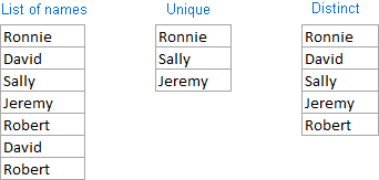
- Unique values - these are the values that appear in the list only once.
- Distinct values - these are all different values in the list, i.e. unique values plus 1st occurrences of duplicate values.
The following screenshot demonstrates the difference:
And now, let's see how you can count unique and distinct values in Excel using formulas and PivotTable features.
How to count unique values in Excel
Here's a common task that all Excel users have to perform once in a while. You have a list of data and you need to find out the number of unique values in that list. How do you do that? Easier than you may think :) Below you will find a few formulas to count unique values of different types.
Count unique values in a column
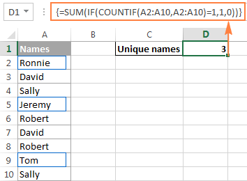
Supposing you have a column of names in your Excel worksheet, and you need to count unique names in that column. The solution is to use the SUM function in combination with IF and COUNTIF:
Note. This is an array formula, so be sure to press Ctrl + Shift + Enter to complete it. Once you do this, Excel will automatically enclose the formula in {curly braces} like in the screenshot below. In no case should you type the curly braces manually, that won't work.
In this example, we are counting unique names in range A2:A10, so our formula takes the following shape:
=SUM(IF(COUNTIF(A2:A10,A2:A10)=1,1,0))
Further on in this tutorial, we are going to discuss a handful of other formulas to count unique values of different types. And because all those formulas are variations of the basic Excel unique values formula, it makes sense to break down the above formula, so you can fully understand how it works and tweak it for your data. If someone is not interested in technicalities, you can skip right to the next formula example.
How the Excel count unique values formula works
As you see, 3 different functions are used in our unique values formula - SUM, IF and COUNTIF. Looking from the inside out, here's what each function does:
- The COUNTIF function counts how many times each individual value appears in the specified range.
In this example,
COUNTIF(A2:A10,A2:A10)returns the array{1;2;2;1;2;2;2;1;2}. - The IF function evaluates each value in the array returned by COUNTIF, keeps all 1's (unique values), and replaces all other values with zeros.
So, the function
IF(COUNTIF(A2:A10,A2:A10)=1,1,0)becomesIF(1;2;2;1;2;2;2;1;2) = 1,1,0,which turns into the array{1;0;0;1;0;0;0;1;0}where 1 is a unique value and 0 is a duplicate value. - Finally, the SUM function adds up the values in the array returned by IF and outputs the total number of unique values, which is exactly what we wanted.
Tip. To see what a specific part of your Excel unique values formula evaluates to, select that part in the formula bar and press the F9 key.
Count unique text values in Excel
If your Excel list contains both numerical and text values, and you want to count only unique text values, add the ISTEXT function to the array formula discussed above:
=SUM(IF(ISTEXT(A2:A10)*COUNTIF(A2:A10,A2:A10)=1,1,0))
As you know, the Excel ISTEXT function returns TRUE if an evaluated value is text, FALSE otherwise. Since the asterisk (*) works as the AND operator in array formulas, the IF function returns 1 only if a value is both text and unique, 0 otherwise. And after the SUM function adds up all 1's, you will get a count of unique text values in the specified range.
Don't forget to press Ctrl + Shift + Enter to correctly enter the array formula, and you will get a result similar to this:
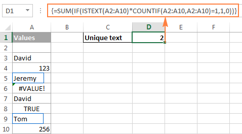
As you can see in the screenshot above, the formula returns the total number of unique text values, excluding blank cells, numbers, logical values of TRUE and FALSE, and errors.
Count unique numeric values in Excel
To count unique numbers in a list of data, utilize an array formula like we've just used for counting unique text values, with the only difference that you embed ISNUMBER instead of ISTEXT in your unique values formula:
=SUM(IF(ISNUMBER(A2:A10)*COUNTIF(A2:A10,A2:A10)=1,1,0))
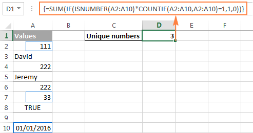
Note. Since Microsoft Excel stores dates and times as serial numbers, they are also counted.
Count case-sensitive unique values in Excel
If your table contains case-sensitive data, the easiest way to count unique values would be creating a helper column with the following array formula to identify duplicate and unique items:
=IF(SUM((--EXACT($A$2:$A$10,A2)))=1,"Unique","Dupe")
And then, use a simple COUNTIF function to count unique values:
=COUNTIF(B2:B10, "unique")
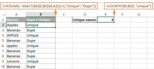
Count distinct values in Excel (unique and 1st duplicate occurrences)
To get a count of distinct values in a list, use the following formula:
Remember, it's an array formula, and therefore you should press the Ctrl + Shift + Enter shortcut instead of the usual Enter keystroke.
Alternatively, you can use the SUMPRODUCT function and complete the formula in the usual way by pressing the Enter key:
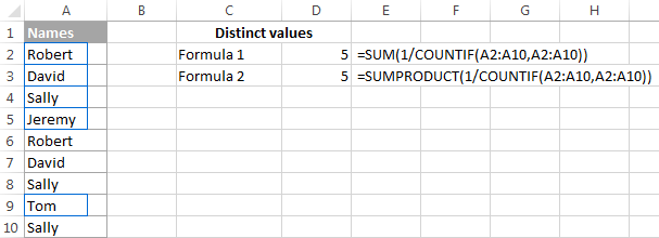
For example, to count the distinct values in range A2:A10, you can go with either:
=SUM(1/COUNTIF(A2:A10,A2:A10))
Or
=SUMPRODUCT(1/COUNTIF(A2:A10,A2:A10))
How the Excel distinct formula works
As you already know, we use the COUNTIF function to find out how many times each individual value appears in the specified range. In the above example, the result of the COUNTIF function is the following array: {2;2;3;1;2;2;3;1;3}.
After that, a number of division operations are performed, where each value of the array is used as a divisor with 1 as the dividend. This turns all duplicates values into fractional numbers corresponding to the number of duplicate occurrences. For example, if a value appears 2 times in the list, it generates 2 items in the array with a value of 0.5 (1/2=0.5). And if a value appears 3 times, it produces 3 items in the array with a value of 0.3(3). In our example, the result of 1/COUNTIF(A2:A10,A2:A10)) is the array {0.5;0.5;0.3(3);1;0.5;0.5;0.3(3);1;0.3(3)}.
Doesn't make much sense so far? That's because we haven't applied the SUM / SUMPRODUCT function yet. When one of these functions adds up the values in the array, the sum of all fractional numbers for each individual item always yields 1, no matter how many occurrences of that item exist in the list. And because all unique values appear in the array as 1's (1/1=1), the final result returned by the formula is the total number of all different values in the list.
Formulas to count distinct values of different types
As is the case with counting unique values in Excel, you can use variations of the basic Excel count distinct formula to handle specific value types such as numbers, text, and case-sensitive values.
Please remember that all of the below formulas are array formulas and require pressing Ctrl + Shift + Enter.
Count distinct values ignoring empty cells
If a column where you want to count distinct values might contain blank cells, you should add an IF function that will check the specified range for blanks (the basic Excel distinct formula discussed above would return the #DIV/0 error in this case):
For example, to count distinct values in range A2:A10, use the following array formula:
=SUM(IF(A2:A10<>"",1/COUNTIF(A2:A10, A2:A10), 0))

Formula to count distinct text values
To count distinct text values in a column, we'll be using the same approach that we've just used to exclude empty cells.
As you can easily guess, we will simply embed the ISTEXT function into our Excel count distinct formula:
And here's a real-life formula example:
=SUM(IF(ISTEXT(A2:A10),1/COUNTIF(A2:A10, A2:A10),""))
Formula to count distinct numbers
To count distinct numeric values (numbers, dates and times), use the ISNUMBER function:
For example, to count all different numbers in range A2:A10, use the following formula:
=SUM(IF(ISNUMBER(A2:A10),1/COUNTIF(A2:A10, A2:A10),""))
Count case-sensitive distinct values in Excel
Similarly to counting case-sensitive unique values, the easiest way to count case-sensitive distinct values is to add a helper column with the array formula that identifies unique values including first duplicate occurrences. The formula is basically the same as the one we used to count case-sensitive unique values, with one small change in a cell reference that makes a great difference:
=IF(SUM((--EXACT($A$2:$A2,$A2)))=1,"Distinct","")
As you remember, all array formulas in Excel require pressing Ctrl + Shift + Enter.
After the above formula is finished, you can count "distinct" values with a usual COUNTIF formula like this:
=COUNTIF(B2:B10, "distinct")
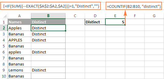
If there is no way you can add a helper column to your worksheet, you can use the following complex array formula to count case-sensitive distinct values without creating an additional column:
=SUM(IFERROR(1/IF($A$2:$A$10<>"", FREQUENCY(IF(EXACT($A$2:$A$10, TRANSPOSE($A$2:$A$10)), MATCH(ROW($A$2:$A$10), ROW($A$2:$A$10)), ""), MATCH(ROW($A$2:$A$10), ROW($A$2:$A$10))), 0), 0))
Count unique and distinct rows in Excel
Counting unique / distinct rows in Excel is akin to counting unique and distinct values, with the only difference that you use the COUNTIFS function instead of COUNTIF, which lets you specify several columns to check for unique values.
For example, to count unique or distinct names based on the values in columns A (First Name) and B (Last Name), use one of the following formulas:
Formula to count unique rows:
=SUM(IF(COUNTIFS(A2:A10,A2:A10, B2:B10,B2:B10)=1,1,0))
Formula to count distinct rows:
=SUM(1/COUNTIFS(A2:A10,A2:A10,B2:B10,B2:B10))

Naturally, you are not limited to counting unique rows based only on two columns, the Excel COUNTIFS function can process up to 127 range/criteria pairs.
Count distinct values in Excel using a PivotTable
The latest versions of Excel 2013 and Excel 2016 have a special feature that allows counting distinct values automatically in a pivot table. The following screenshot gives an idea of how the Excel Distinct Count looks like:
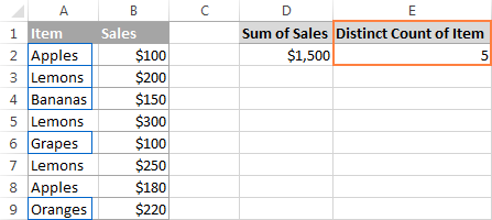
To create a pivot table with the distinct count for a certain column, perform the following steps.
- Select the data to be included in a pivot table, switch to the Insert tab, Tables group, and click the PivotTable button.
- In the Create PivotTable dialog, choose whether to place your pivot table in a new or existing worksheet, and be sure to select the Add this data to the Data Model checkbox.

- When your pivot table opens, arrange the Rows, Columns and Values areas the way you want. If you don't have much experience with Excel pivot tables, the following detailed guidelines may prove helpful: Creating a PivotTable in Excel.
- Move the field whose distinct count you want to calculate (Item field in this example) to the Values area, click on it, and select Field Value Settings… from the drop-down menu:

- The Value Field Settings dialog window will open, you scroll down to Distinct Count, which is the very last option in the list, select it and click OK.
You can also give a custom name to your Distinct Count if you want to.

Done! The newly created pivot table will display the distinct count like shown in the very first screenshot in this section.
Tip. After updating your source data, remember to update the PivotTable to bring the distinct count up to date. To refresh a pivot table, just click the Refresh button on the Analyze tab, in the Data group.
This is how you count distinct and unique values in Excel. If someone wants to have a closer look at the formulas discussed in this tutorial, you are welcome to download the sample Excel Count Unique workbook.
I thank you for reading and hope to see you again next week. In the next article, we are going to discuss various ways to find, filter, extract and highlights unique values in Excel. Please stay tuned!
 by
by
225 comments
I'm sorry that the formula was in my own language - here it is in the English version:
=SUM(IF(FREQUENCY(IF(SUBTOTAL(3;OFFSET($D$9;ROW($D$9:$D$2000)-ROW($D$9);;1));IF($D$9:$D$2000"";MATCH($D$9:$D$2000;$D$9:$D$2000&"";0)));ROW($D$9:$D$2000)-ROW($D$9)+1);1))
I have an autofiltered column with different week numbers from 1 to 52 and from this I want to calculate the distinct number of filtered week numbers. Let's say I have excluded all week numbers higher than 5 and have the followning rows shown:
1
1
2
3
3
3
5
I have tried to calculate the number of distinct weeks (4) with use of this formula which was entered with Ctrl-Shift-Enter:
=SUM(HVIS(FREKVENS(HVIS(SUBTOTAL(3;FORSKYDNING($D$9;RÆKKE($D$9:$D$2000)-RÆKKE($D$9);;1));HVIS($D$9:$D$2000"";SAMMENLIGN($D$9:$D$2000;$D$9:$D$2000&"";0)));RÆKKE($D$9:$D$2000)-RÆKKE($D$9)+1);1))
Unfortunately, it seems like this formula only work with text values and not with week number even I have formatted the cells as text.
Therefore, I will appreciate to hear from you what I can do.
Hello!
I hope you have studied the recommendations in the tutorial above. It contains answers to your question.
To count distinct values you can use this array formula:
=SUM(IF(A1:A20<>"",1/COUNTIF(A1:A20, A1:A20), 0))
Thank you for the tip.
I have tried the formula and it works fine. But when I use it in a column with autofilter, all rows are included in the calculation - even the rows that are not included in the filter.
Is it possible to adjust the formula so that only the filtered rows are included in the calculation, as it e.g. done in Subtotal (9; range)?
In my example, the formula should show 3 if week 5 is not included in the filter.
Hello!
Unfortunately, the SUBTOTAL and AGGREGATE functions do not work with arrays. They only work with cell ranges. Therefore, you can write on a separate column the array formula (for example, in cell L1)
=IF(SUM((EXACT($A1:$A$1,$A1)*($A1<>"")))=1,1,"")
This is an array formula and it needs to be entered via Ctrl + Shift + Enter, not just Enter. After that, you can copy this formula down along the column.
To count distinct values that are not hidden by the filter, use the formula
=AGGREGATE(9,5,L1:L50)
I hope it’ll be helpful.
Hello,
Below is sample data for a limo service company. My goal is to write a formula to count the number of distinct drivers that drove on a given day with certain criteria (see example criteria below)
Example Criteria: Confirmed: Yes, Paid: Yes, Size purchased: Sedan
We can pretend my data is A2 to E13 below:
Date Confirmed? Paid? Size purchased Driver
1/1/2022 Yes Yes Sedan Bob
1/1/2022 Yes Yes SUV Joe
1/1/2022 No No SUV Joe
1/1/2022 Yes Yes Sedan Mike
1/1/2022 Yes Yes Sedan Matt
1/1/2022 Yes Yes SUV Joe
1/1/2022 Yes No Sedan Bob
1/2/2022 No No Sedan Bob
1/2/2022 Yes Yes Sedan Bob
1/2/2022 Yes Yes SUV Joe
1/2/2022 Yes No SUV Steve
1/3/2022 Yes No Sedan Bob
1/3/2022 Yes Yes Sedan Bob
The answer based on the below would be 3 for 1/1/2022 (Bob, Joe and Matt). Bob drove two different customers on 1/1/2022 and Joe and Matt each drove 1, but since I'm looking for distinct count, I only want Bob's name once. I thought I had this solved in a pivot table, but it's not producing the correct answers and a formula would be much easier for the particular report I am producing. Thank you in advance!
Correction: the correct names would be Bob, Mike and Matt (not Joe since Joe's in a SUV). Apologies
Hello!
Your data example does not match the description. You can try the formula
=COUNTIFS(B2:B14,"Yes",C2:C14,"Yes",D2:D14,"Sedan",A2:A14,"="&"01.01.22")
It gives the result - 3.
If you want to count the number of unique values in column E, use this formula
=COUNTA(UNIQUE(FILTER(E2:E14,(B2:B14="Yes")* (C2:C14="Yes")*(D2:D14="Sedan")* (A2:A14=DATEVALUE("01.01.22")))))
You can find detailed instructions and examples in this article: How to count unique values in Excel with criteria.
I hope it’ll be helpful.
Is it possible to achieve this in excel 2016?
I have this data and need to do a distinct count of company name where column B is NOT blank
Company Criteria
Company A Yes
Company B Yes
Company C
Company D Yes
Company A
Company C Yes
Company A Yes
Company B
Hello!
These functions are not available in Excel 2016. You can get a list of unique values in a separate table, as described in the article: How to get a list of unique and distinct values in Excel.
Then count them with the COUNTA or COUNTIF function
Good morning,
I'm working on the EEO-4 data report and trying to pull the data without having to manually count how many employees fit the criteria I'm being asked to report on. I've tried using a pivot table and the countifs function but cant seem to quit get it to work. I need to look at 1. Job category, ethnicity, gender and salary range and list how many employees fall under that category.
Ex: How many male technicians make between $55 - $69,999?
The report has a salary band that is making it difficult for me to group the salaries by lets say $5k, $10K, etc. Range I need to use is below.
$0.1 - $15.9
$16.0 - $19.9
$20.0 - $24.9
$25.0 - $32.9
$33.0 - $42.9
$43.0 - $54.9
$55.0 - $69.9
$70.0 PLUS
How can I use a pivot table or formula/both to quickly fill in this chart? Do I need to change the format of my spreadsheet in a way that is easier to use a formula? There are multiple job categories, multiple salary ranges, and multiple ethnicities. My excel spreadsheet has the exact job category, salary and ethnicity for each employee.
Hello!
To count the number of employees for a condition, you can use the COUNTIFS function. You can find the examples and detailed instructions here: Excel COUNTIFS and COUNTIF with multiple AND / OR criteria.
This should solve your task.
Hi. How to count the number of dates in the cell for a specific name in another cell?
e.g:
SALESPERSON DATE TO CUSTOMER TOTAL NO. OF DATES THE SPECIFIC SALESPERSON SEND OUT
cindy 11/11/2021 =(TOTAL NO. OF DATES CINDY SENT OUT)
cindy 15/11/2021
cindy 18/11/2021
cindy 21/11/2021
alan 1/11/2021 =(TOTAL NO. OF DATES ALAN SENT OUT)
alan 2/11/2021
alan 3/11/2021
alan 4/11/2021
shane 17/11/2021 =(TOTAL NO. OF DATES SHANE SENT OUT)
shane 18/11/2021
Hello!
If I understand your task correctly, Here is the article that may be helpful to you: Count unique values with criteria.
Hope you’ll find this information helpful.
Could you pls advise how to calculate the following with easiest method.
A B C D E F G H I
1 X IX III II V I V VII II
2 IX VIII I VI IV X III II V
3 IX VIII I VI IV X III II V
4 V I X IX I II V V VI
5 VII II X II III IV V VIII I
6 VIII III IX IX I II VII V VII
Actually I want to calculate how many period a teacher is taking in each class in a week.
Hope your reply soon.
Hello!
I do not see a teacher in your data. However, I recommend using the COUNTIF function to conditionally calculate the quantity.
I am still struggling with a concise way to count unique values in a column based on the values in another column. For example, let's say I want to count the unique occurrences of a name in Column A based on Column B containing the keyword "count". Say that this is my data in A1:B6:
Robert count
Mitch
David
Jeremy count
Robert count
David count
The desired output is 3, because there are 3 unique names marked "count". However, the array formula ={SUM(IF(B1:B6 = "count", 1/COUNTIF(A1:A6, A1:A6), 0))} returns 2.5, because the unmarked David is included in the COUNTIF denominator. What would be the right formula to do what I'm trying to do?
Hello!
You can learn more about counting unique values with criteria in Excel in this article on our blog.
=IFERROR(ROWS(UNIQUE(FILTER(A2:A10,B2:B10="count"))), 0)
This should solve your task.
Is there any excel formula where the distinct count and count if formula numbers should match..If count if formula used its splits the decimals based on same items , i dont want to splt that.
I have a key combination (ID+Dept)
Can some help
Hi!
What do you want to calculate exactly? Your question is not entirely clear, please specify.
Is there any excel formula where we can get count as same as using distinct pivot table.
Hello!
Please have a look at this article — Excel SUBTOTAL function with formula examples
I hope it’ll be helpful.
Hi
The formula you give
=IF(A1 < TODAY(),"", A1-TODAY())
is not showing the minus number of day or days
and this below
=IF(ISBLANK(A1),"",A1-TODAY())
is working but I want the result cell will show with the text Day or Days including the Numbers. For example, 2 Days, 1 Day, -1Day, -3 Days & I want Zero Day will not show, or the cell (Zero Day) will blank.
Please also suggest how to share my excel file with you.
My second question is the subtraction of two dates comes zero (A1-A2=0) I want the cell will show the text "Same Day" and if A1 & A2 is blank result will show also blank, hope you understand, thanks in advance.
Regards
Sazedul Munna
Hello!
I recommend reading this guide: Date difference in days, months and years.
I hope I answered your question. If something is still unclear, please feel free to ask.
Hi
I tried many ways but I can't get my expected result. I can't get the number including text Day or Days, For example, 2 Days, 1 Day, -1Day, -3 Days & I want Zero Day will not show, or the cell (Zero Day) will blank. I would like to share my excel file with you to solve these.
Thanks
Sazedul Munna
Hi
This is Sazedul from Bangladesh, I face some problems of my own sheet when I'm working on it if I get support from you will develop the sheet of my own style. Problems are as follows -
A) How can I count a number which is the double number, I have these numbers (1,2,3,4,5,11,23) and my problem is, the double number is counted separately. Instead of 7 it counted 9. Here I use this formula
=SUM(LEN(A1)-LEN(SUBSTITUTE(A1,2,3,4,5,6,7,8,9,0},)))
B)
FABRIC REC DATE FABRIC FOLD DATE DURATION
06-Mar-21 12-Apr-21 37 Days
15-Mar-21 15-Mar-21 Same Day
08-Mar-21 12-Mar-21 04 Days
#VALUE!
15-Apr-21 19-May-21 34 Days
#VALUE!
#VALUE!
#VALUE!
Here I want a DURATION of FABRIC FOLD DATE & FABRIC REC DATE
as you see in the above. But result in these blank cell shows #VALUE!
In DURATION Column I use this formula
=IF([@[FABRIC FOLD DATE]]-[@[FABRIC REC DATE]]=0,"Same Day",[@[FABRIC FOLD DATE]]-[@[FABRIC REC DATE]])
How do I solve this?
C)
REMAIN DAYS MONTH STATUS GD RECEIVED ALLOTED GREIGE DATE
4 Days May-21 In Progress 06-May-2021 15 Days 21-May-2021
10 Days May-21 Complete 12-May-2021 15 Days 27-May-2021
5 Days Apr-21 Delayed 12-Apr-2021 40 Days 22-May-2021
-6 Days Apr-21 Not Started 16-Apr-2021 25 Days 11-May-2021
15 Days May-21 Delayed 17-May-2021 15 Days 01-Jun-2021
#VALUE! Complete
#VALUE! Delayed
#VALUE! Not Started
Here I Want if GREIGE DATE column is blank REMAIN DAYS will blank but I can’t make it.
In REMAIN DAYS Column I use this formula
=Reoprt[@[GREIGE DATE]]-TODAY() {Here Report is the Table name}
Please help me to resolve these & will be grateful to you.
Best Regards
Sazedul Munna
Hello!
If your numbers in the text are separated by commas, use the formula
=LEN(A1)-LEN(SUBSTITUTE(A1,",",""))+1
You will count how many numbers are in the text.
Question B is not clear to me.
To avoid subtracting the current date from an empty cell, use the formula
=IF(A1 < TODAY(),"", A1-TODAY())
or
=IF(ISBLANK(A1),"",A1-TODAY())
I hope it’ll be helpful.
Thanks for your reply, but it's not working
Hi!
What exactly isn't working?
Hi
Extremely sorry actually it's my mistake, your formula is working....
=LEN(A1)-LEN(SUBSTITUTE(A1,",",""))+1
In the excel table there shows 1 if the formula is put my question is how can I keep the cell blank, thanks in advance.
I have another question suppose in a cell I want subtraction of two dates and result comes Zero Day or 1 Day or 2 Days or Minus 1 Day or Minus 2 Days. How do the cells show Day or Days including the Numbers as mentioned? For example, 2 Days, 1 Day, -1Day, -3 Days & I want Zero Day will not show or the cell (Zero Day) will blank. How can I do this?
Regards
sazedul Munna
Hi!
I have already answered this question.
Hello!
Suppose if in column A text is given i want duplicate will give same Previous No and unique text will be sum of highest no
eg.
C-A C-B
XYZ - 1
ABC - 2
CDE - 3
XYZ - 1
DEF - 4
ABC - 2
DEF - 4
*Column-A is text & Column B i want
Can you pls help me t
Hello!
Your list should start in cell A2. Suppose your data are in column A, please try to enter the following formula in cell B2 and then copy it down along the column:
=IF(COUNTIF($A$1:A2,A2)=1, MAX($B$1:B1)+1, INDEX($B$1:B1,MATCH(A2,$A$1:A2,0)))
This should solve your task.
Hi,
I am giving below the sample data for understanding. I want the course wise unique count of the student. Can you pls help me to get it through count unique formula?
Sample Data:
Student Name Course
Ajay NID
Vijay NIFT
Nilesh NID + NIFT
Mahesh NIFT
Ajay NID + NIFT
Vidya ARCH
Sudha NID + NIFT
Amit NID
Siddhesh ARCH
Thanks.
Narendra
Per your response, below is a sample of data and desired query.
DATA
| A | B | C | D | E |
1 | NAME | CREDIT | REF DATE | ADM DATE | SHARED R/AA |
2 | N1 | .05 | 01/02/21 | 01/03/21 | Y |
3 | N2 | .05 | 01/02/21 | 01/03/21 | YY |
4 | N3 | 1 | 01/02/21 | 01/03/21 | |
5 | N1 | .05 | 01/02/21 | | Y |
6 | N1 | .05 | 01/02/21 | | Y |
(LINE 1 A-E are the headers)
(LINES 2-6 A-E is the data)
QUERY RESULTS NEEDED (based on data above)
REFERRALS BY NAME (results)
FORMULA attempted for NAME N1:
=countifs(A2:A6,"N1", B2:B6 "sum", E2:E6, "Y" or "empty") result should be 1.5
FORMULA attempted for NAME N2:
=countifs(A2:A6,"N2", B2:B6 "sum", E2:E6, "Y" or "empty") result should be 0.5
FORMULA attempted for NAME N3:
=countifs(A2:A6,"N3", B2:B6 "sum", E2:E6, "Y" or "empty") result should be 1
ADMITS BY NAME (results)
FORMULA attempted for NAME N1:
=countifs(A2:A6,"N1", B2:B6 "sum", E2:E6, "YY" or "empty") result should be 0.5
FORMULA attempted for NAME N2:
=countifs(A2:A6,"N2", B2:B6 "sum", E2:E6, "YY" or "empty") result should be 0.5
FORMULA attempted for NAME N3:
=countifs(A2:A6,"N3", B2:B6 "sum", E2:E6, "YY" or "empty") result should be 1
Obviously, my logic is wrong. I hope this clarifies my desired results.
With thanks,
Bob
Hi,
The COUNTIFS function counts the number of values. Therefore, the result of its calculations can only be an integer. I am assuming that you want to calculate the amount. So use the SUMIFS function.
Perhaps this formula will work for you.
=SUMIFS(B2:B6,A2:A6,"N1",E2:E6,"Y") + SUMIFS(B2:B6,A2:A6,"N1",E2:E6,"")
However, I don't understand how you want the result 1.5 if the sum of all the numbers is 1.2.
You can learn more about SUMIFS in Excel in this article on our blog.
You can learn more about COUNTIFS in this guide.
Greetings
I'm in need of guidance on the following:
I need to get a count of two columns of data:
COLUMN A is the credit for a referral, that referral has a value of 0 or .5 or 1
COLUMN B is the date of the referral and if shared (e.g: the .5 from COLUMN A) will show twice.
I have attempted COUNTIFS but just get a total of COLUMN B or an ERROR when criteria for COLUMN A is included.
Hoping someone can help.
Bob
Hello!
Your task is not completely clear to me. Unfortunately, without seeing your data it is difficult to give you any advice. Please provide me with an example of the source data and the expected result.
Hello,
I want unique count of patient by location. I know how to do this using Pivot, but i don't know how to do this with excel formulas.
Hello!
Please check out the following article on our blog, it’ll be sure to help you with your task: Count unique values with criteria
Hope you’ll find this information helpful.
Hi,
I have one row of data containing some items, and another row of data containing those items again. I need to see how many of them are repeated in the second row, excluding duplicates. There may be blanks also but they should not be part of the output.
e.g. row 1: {a,b,c,c,d,e,f,g,g}
row 2: {a,c,d,d,e,g,h}
Output should be 5 (i.e. a,c,d,e,g are repeated in row 2).
Thanks a lot for helping.
Hi friend..
Need your support in excel
Column D contain n' number of cities names
Column E contain some numeric values (numbers contain only in few cells of column E but not all)
Can you please help me in framing a excel formula to count unique values in column D (count cities) where numeric value in column E is greater than ZERO
One city may repeat in column D and have values in column E but the city would be counted as one only
This is my request
Thank You!
I've a requirement which i'm unable to figure out.
There are dates in a column, names in another column, product IDs in another column.
Names & product ID's would repeat.
How to create a crosstab report with names as colum header, month as row header & count of distinct product IDs as data fulfilling the headers.
Thanks in advance.. :)
Hello!
Please check out the following article on our blog, it’ll be sure to help you with your task: How to make and use PivotTables in Excel
I hope it’ll be helpful.
I have a simple problem, but I cannot get my head round how to do it, and not found an answer on the web.
I have a column of multiple entries of 1000 mixed up products. Each product has a column with a quantity.
So OK its easy to sort products, using inbuilt 'sort' on a column.
The next bit I fail on. I have tried a lot of variants of countif.
A - 2
A - 4
B - 5
B - 6
I want a result as follows
A - 6
B - 11
Any ideas please.
Hello!
Please check out the following article on our blog, it’ll be sure to help you with your task: How to use SUMIF function
Hope you’ll find this information helpful.
What if some of my text that I want to distinct count are more than 255 characters long? The limit of the COUNTIF function is that it processes only characters that are less than 255 characters, otherwise the formula would return a #VALUE!. Is there a workaround for this problem? Hope you can help.
Hello!
The SEARCH function does not have the same restrictions as the COUNTIF function. If I understand the problem correctly, you can use the formula to count matches in long text:
=SUM(--ISNUMBER(SEARCH("Text to find",A2:A100,1)))
I hope my advice will help you solve your task.
Thanks for the reply Alexander. But I need a formula that distinct counts a column of text wherein some texts are more than 255 characters long. The formula that you gave does not seem to give the right total count.
Hello!
The formula I sent to you was created based on the description you provided in your first request. However, as far as I can see from your second comment, your task is now different from the original one.
This formula will return TRUE if there is a cell longer than 250 characters in the column.
=IF(SUM(--(LEN(A1:A1000)>250))>0,TRUE)
Alexander,
i really appreciate your help. Thank you.
2020 January Nick
2020 January Nick
2020 January Nick
2020 January Jim
2020 February Adam
2020 February Adam
2020 February Adam
2020 February Adam
2020 February Nick
2020 February Jim
i apologize that i didnt clearly state what i was looking for. when i type in the formula that you suggested, it comes back with 0. in the above data, i am trying to figure how many different names or people showed up in January 2020, how many in February 2020, etc. So for January 2020, the result should be 2. and for February 2020, the result 3.
Hello!
Your data changes all the time. For these you can use the formula
=SUMPRODUCT((A1:A10&B1:B10="2020"&"January")/COUNTIFS(B1:B10,B1:B10,C1:C10,C1:C10))
Hope this is what you need.
Dear Alexander
what is the formula if i use range data from A1 until C100, which is the cell is fill until A10:C10 for this moment.
when tomorrow i will fill the data cell from A11:C12
And the day after tomorrw i will fill data cell from A13:C15
Just like the example for this moment the cell fill with data january and february. and tomorrow i fill with march
So i dont need to change range data because the formula has range wider which is until 100 rows.
Thank for your answer.
Dear Alexander
column A11 until C100 is still empty cell
i will not fill it in the same day. i fill it once a day.
the formula can read empty cell
thanks
Hello!
Sorry, I do not fully understand the task. Could you please describe it in more detail? Please specify what you were trying to find, what formula you used and what problem or error occurred. It’ll help me understand your request better and find a solution for you.
2020 Jan Steve
2019 Jan Mike
2020 Feb John
2018 Mar Nick
2020 Feb Mike
2020 Feb Mike
2019 Jan Steve
that formula doesnt seem to be working. The above data is a sample of what i am working with. i am trying to figure out how many different people showed up on a particular year and month. There are going to be many duplicate first names that i only want counted one time. hope you can help!
Hello!
I wrote this formula based on the description you provided in your original comment. Please note that if you’d provided me with the precise and detailed description of your task from the very beginning, I’d have created a different formula that would have worked for your case.
However, if you write that the formula does not work, but do not say what exactly does not work, I cannot help you. I will not guess your desires. What result do you want to get?
For your data, you can replace the month number 2 with "Feb". I think it's not difficult.
i have 3 columns of data. The first column is the Year, the 2nd column is the month, and the 3rd column is a list of First names. im trying to create a formula that would count for example how many DIFFERENT names appear in February 2019. Can someone please help??
Hello!
The formula below will do the trick for you:
=SUM(IF(COUNTIFS(C1:C10,C1:C10,B1:B10,2,A1:A10,2019)=1,1,0))
The formula counts the number of unique rows that match the conditions.
Hi, i have tried the recommendations given but don't seem to make head way.
i have a database with several columns including
1. state (44 distinct locations with several duplicates)
2. Ward ( more than 1 state can have the same name for different wards but no two wards in same state have same name)
3. Outcomes ( Yes or No)
I want to count distinct wards (dublicate is only when state and ward is same) that have "yes" as outcome.
Please help.
Thank you so much, its help me a lot. I am impressed on this article.
Hi,
This was very useful, but I am having some issues:
1) I have column A as the month (1=Jan, 1=Feb, etc), and column B as the Client. When counting TOTAL distinct clients for the entire year (ie all months), how can I adjust the formula so it does not count cell B1 (the header/name of column), and updates dynamically as more data is added to the raw data sheet?
2) How can I adjust this formula so I can find # distinct clients broken down by month, updated dynamically as more data is added?
Thank you!
Hello Olivia!
To count the number of unique values in column B, use the instructions provided earlier in this article. Specify the counting range large, for example B2: B9999
To calculate the number of unique customers per month, use the additional condition - the number of the month.
If the month number = 2, then you can use something like this formula
=SUM(IF(ISTEXT(B2:B100)*(--IF(A2:A100=1,1,0))*COUNTIF(B2:B100,B2:B100)=1,1,0))
I hope it’ll be helpful.
Hello,
I'm creating a data table with that shows the count of people in each expertise level. The count is created by a 'COUNTIFS' formula. Formula looks as follow:
=(IF(COUNTIFS(SkillsetData!B:B,IndustryExpert_ORTEMS_CSVREADY!B2,SkillsetData!CP:CP,">0",SkillsetData!AD:AD,IndustryExpert_ORTEMS_CSVREADY!$L$2)=0,"",(COUNTIFS(SkillsetData!B:B,IndustryExpert_ORTEMS_CSVREADY!B2,SkillsetData!CP:CP,">0",SkillsetData!AD:AD,IndustryExpert_ORTEMS_CSVREADY!$L$2))))
The next challenge is to base the count on unique values. I have one column called "name' (A) with duplicates in it. Now I am looking for a solution to integrate a formula in the existing formula that only counts the unique 'name' from column A before starting to look at the other criteria in the COUNTIFS formula.
I really appreciate your help.
Have a nice day!
Hello Erik!
Unfortunately, without seeing your data it is impossible to give you advice.
I'm sorry, it is not very clear what result you want to get. Could you please describe your task in more detail and send us a small sample workbook with the source data and expected result to support@ablebits.com? Please shorten your tables to 10-20 rows/columns and include the link to your blog comment.
We'll look into your task and try to help.
Hello Alexander,
Thank you for your reply. I did some more research today and I have found a way to create the result that I was looking for. I needed to define per row if there are any duplicated based on two columns (without removing the data). I found a nice trick with a reverse COUNTIFS formula. Starting from the bottom and dragging it up.
Anyway thanks for your reply and offer to help!
Have a nice day.
Good day,
could you support me with a solution for a such output : the result should be at the end of the list (the last cell), I have huge list of columns and I need to know the distribution of each one, without passing through Pivot table:
Item
0
0
11
11
11
11
4
4
4
6
6
6
6
0(2),11(4),4(3),6(4)
Thank you!
Hello!
I recommend this article: How to get a list of unique and distinct values in Excel
Hi,
I have a question about my excel datasheet. In column A i have audit partner names and in column B i have different issuer cik numbers. I want to count how many different companies one audit partner audits. So, how many audit clients one audit partner has. Is there an excel formula for this?
Kind regards,
Rohan Kapoor
Hello Rohan!
I could help you if I knew what "issuer cik numbers" are. If you give an example of your data, I will try to help you. Please describe your problem in more detail. It’ll help me understand it better and find a solution for you. Thank you.
I have a spredsheet having column A with repeated names. The an other column B contains the month. One more column C contains some text like fresh/renewal/enhancement. I need to count unique text or names entered in Column A, with criteria if month in column B is "MAY" and Column C contains text "Fresh". the formula should works If there is blank cell also and if we added the data frequently at below.
Hello!
If I understand your task correctly, to calculate the number of unique values by conditions, use the formula:
=SUMPRODUCT(--(B2:B17="MAY"), --(C2:C17="Fresh"), --($A$2:$A$17=A2))
I hope this will help
I want to count the number of unique values based on the string in the cell and the format as my data is distingquished by format. So if I have 50 SAC 25 blue and 43 green. It would be counted as 2 in the occurances.
Hello Jeffrey!
I recommend to study the article How to count cells by color in Excel
Describe your problem in more detail. Include an example of the source data and the result you want to get. It’ll help me understand your request better and find a solution for you. Thank you.
Hi,
I have 2 Columns with different range
column G - column H
Rock Grades - Surveyed Qty
1-500 kg - 3,411
1-1000 kg - 8,673
300-1000 kg - 11,757
60-300 Kg - 3,001
750 mm - 7,916
60-300 Kg 4,186
I want a formula how to calculate these Rock Grade values with particular categories wise
Hello!
I’m sorry but your task is not entirely clear to me.
What exactly do you want to count? For me to be able to help you better, please describe your task in more detail. It’ll help me understand it better and find a solution for you. Thank you.
Hi, I’m looking for a formula to count unique reference numbers which contains both numbers and letters, example 12345 MCP107 in the cell range E2:E57 only if meets the criteria of “N” in the range G2:G57. I am using excel 2010 - can you help me out with this please?
I am using this formula to count how many times a particular word appear within a range of cells, and it works...however I need to include additional characters after the particular word (example: "candidate 10/10")
=SUMPRODUCT((LEN(range)-LEN(SUBSTITUTE(range, "candidate","")))/LEN("candidate"))
Hello, I apologize in advance for asking for help but hopefully, this is an easier one for you, less so for me.
I have a large data set with one unique identifier, that being the VIN number of a vehicle. When we process a service transaction for a vehicle, sometimes there will be more than one tech working on the same vehicle and that will require more than one entry into the spreadsheet. To accommodate this requirement I have set up a macro that copies all of the data on the selected row and places a duplicate on the next available row. The problem I have is that in doing so, it creates a duplicate of everything including several items that I don't want to be duplicated such as total job hours and total hours quoted as these will distort the records if my staff fail to remove these manually each time.
What I am trying to achieve is to have a formula that can be used in the total hour's sum cell (B50) that detects the duplicated record created by the macro having detected the VIN as identical to the same VIN already used previously in that column, A1:A50.
The problem I am trying to solve occurs because the entire job hours and job $ values are recorded as a whole when the record is first created. The macro then creates an entirely new duplicate record though artificially doubling the sum value by adding new row with a clone of the same data. I want to keep the clone data as-is but I just don't want to count the additional hours that now appear in the hour's column C1:C50.
I intend to use the same formula for several items including hours and all dollar values for that job as the problem affects several cells. I just need one working formula and I can modify it from there for each column.
I sincerely hope that makes sense.I am happy to send you the sheet if that makes this easiler to understand.
How do you get this formaula to also ignore errors as well as Error values such as "#NUM"
You can use sumif function.
Before that, pls insert new coloumn and enter "1" in to all lines.
And select and copy all names in to new coloumn.and remove the duplicates.and use the sumif function and get the sum of services each patient.
I have two columns. Column A contains 5 different treatments for vehicles, let's say treatments S, T, U, V and W. These five treatments are applied to vehicles in column B. The same vehicle might receive more than one treatment per month, sometimes the same treatment twice. I want to know how many distinct vehicles in column B received treatments S, T and V. Thus distinct values based on multiple OR criteria from the same column A. Typical 2500 to 5000 rows per month.
Please help me with an Excel formula that will solve this problem?
Ps. Thank you, your site has been very helpful to me!
AN EXCEL SHEET CONTAINS DATA
EG:-IN CERTAIN CELLS CONTAIN ONLY A NAME (Eg:- "RONY")
IN CERTAIN CELLS CONTAIN TWO or more NAMES (Eg:- "RONY,SONA")
HOW CAN I COUNT ONLY ONE PARTICULAR NAME IN THAT SHEET using formula?
Dear all,
Request you to kindly help me understand this formula:
=SUM(IFERROR(1/IF($A$2:$A$10"", FREQUENCY(IF(EXACT($A$2:$A$10, TRANSPOSE($A$2:$A$10)), MATCH(ROW($A$2:$A$10), ROW($A$2:$A$10)), ""), MATCH(ROW($A$2:$A$10), ROW($A$2:$A$10))), 0), 0)). I posted a comment earlier as well and it was removed.
Thank you!
Dear all,
Could you please elaborate the working of this formula: "=SUM(IFERROR(1/IF($A$2:$A$10"", FREQUENCY(IF(EXACT($A$2:$A$10, TRANSPOSE($A$2:$A$10)), MATCH(ROW($A$2:$A$10), ROW($A$2:$A$10)), ""), MATCH(ROW($A$2:$A$10), ROW($A$2:$A$10))), 0), 0))".
Thank you in advance!
Dear All,
Please i need help, I want to count unique values with criteria and reported to a general summery to another "sheet".
please advice
Month Agent Sales Agent Status
JAN A 0.02 A 1
JAN B 0.00 B 1
JAN C 0.02 C 1
JAN D 0.03 D 1
JAN E 0.06 E 1
JAN F 0.05 F 1
FEB A 0.00
FEB B 0.00
FEB C 0.04
FEB D 0.02
FEB E 0.01
FEB F 0.00
MAR A 0.04
MAR B 0.03
MAR C 0.02
MAR D 0.06
MAR E 0.05
MAR F 0.06
Hi...
Request you to please go thru' the above concern.
We have 6 agents (A,B,C,D,E,F) did sales more than 2k (it's a must) a period of 3 months.
At the end of quarter we wish to know all agents did one time sales i.e.>=2k (either one time or more) or not.
If we have the data like above, please suggest a formula.
A B
00:00 E/F
01:00 E/F
02:00 E/F
03:00 10
04:00 E/F
05:00 E/F
06:00 5
07:00 10
08:00 L/S
09:00 L/S
10:00 L/S
11:00 L/S
12:00 L/S
13:00 L/S
14:00 12
15:00 P/O
16:00 P/O
17:00 P/O
18:00 P/O
19:00 O/C
20:00 O/C
21:00 O/C
22:00 E/F
23:00 E/F
There are 3 sets of E/F here.How will i get excel to output 3 counts? That is 1 count for each set of E/F.Thanks
Hello, Im Trying to create a formula for this one, I need to count distinct values per week, only the “Open” status. The hard part is, you dont need to count the”Open” status if at a certain time that week it was already closed.
SR Reference# Week # Status
19999 32 Closed
189898 32 Open
189898 32 Closed
189898 29 Closed
189898 31 Open
19999 33 Open
19999 33 Open
Thanks in advance!
None of this works. Rubbish article.
Hello Samuel,
You can download our sample workbook and make sure all the formulas work exactly as described.
=IF(ISNUMBER(MATCH("Apples",M:M,0)),COUNTIF(N:N,"Green"),0)
This formula is not perfect. I want to see if there are "Apples" in one column and "Green" in corresponding column, it should count all Green Apples.
Thanks.
Hi,
How can I count unique value within a range IF these values match those of another column? For example, in column A I have Apples, Oranges, Bananas.
In column B I have several types of cars.
How can I count the different types of car associated with each fruit (eg. banana)?