Now, that we've learnt how to enter dates and time to your spreadsheet, it's time to talk about the ways of calculating time in Google Sheets. We'll discuss the ways of finding time difference in detail, see how to sum dates and time together, and learn to display only date or time units and set them apart completely.
How to calculate time difference in Google Sheets
When you're working on some projects, it is usually important to control how much time you spend. This is called elapsed time. Google Sheets can help you calculate the time difference in a lot of various ways.
Example 1. Subtract time to get the time duration in Google Sheets
If you have your start time and end time, it's not a problem to find out the time spent:
Let's assume the start time is in column A and the end time is in column B. With a simple subtraction formula in C2, you will find how much time this or that task took:
=B2-A2
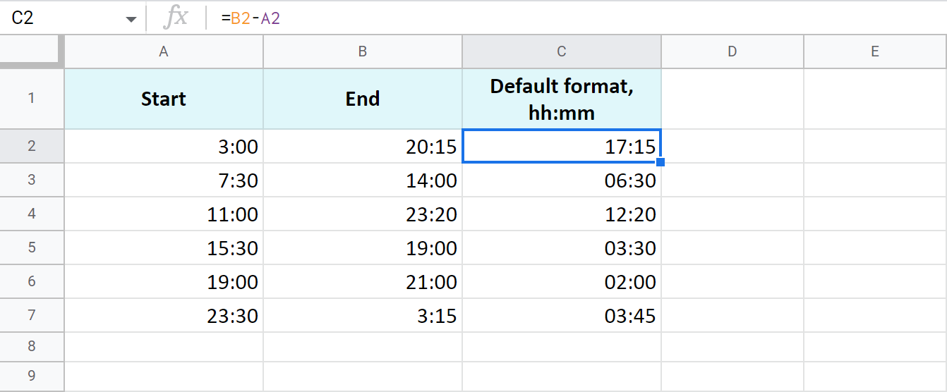
The time is formatted as "hh:mm" by default.
To get the results as hours only or as hours, minutes, and seconds, you need to apply a custom format with the corresponding time codes: h and hh:mm:ss. Google even offers a special number format for cases like this - Duration:
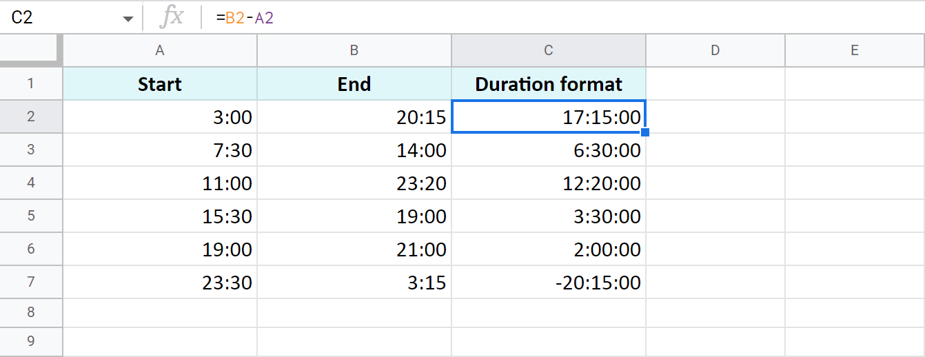
Tip. To apply the custom time format, go to Format > Number > Custom number format in your spreadsheet menu.
Example 2. Calculate time duration in Google Sheets using the TEXT function
Another trick to calculate the time duration in Google Sheets involves the TEXT function:
=TEXT(B2-A2,"h") - for hours
=TEXT(B2-A2,"h:mm") - for hours and minutes
=TEXT(B2-A2,"h:mm:ss") - for hours, minutes, and seconds
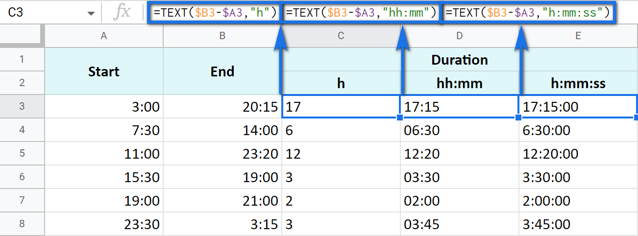
Note. See how the records are aligned to the left? Because the TEXT function always returns the results formatted as a text. This means these values cannot be used for further calculations.
Example 3. Time difference in hours, minutes, and seconds
You can track the time spent and get the result in one time unit disregarding other units. For example, count the number of only hours, only minutes, or only seconds.
Note. To ensure correct results, your cells should be formatted either as numbers or automatically: Format > Number > Number or Format > Number > Automatic.
-
To get the number of hours spent, subtract your start time from the end time and multiply the result by 24 (since there are 24 hours in one day):
=(End time - Start time) * 24You will get a time difference as a decimal:

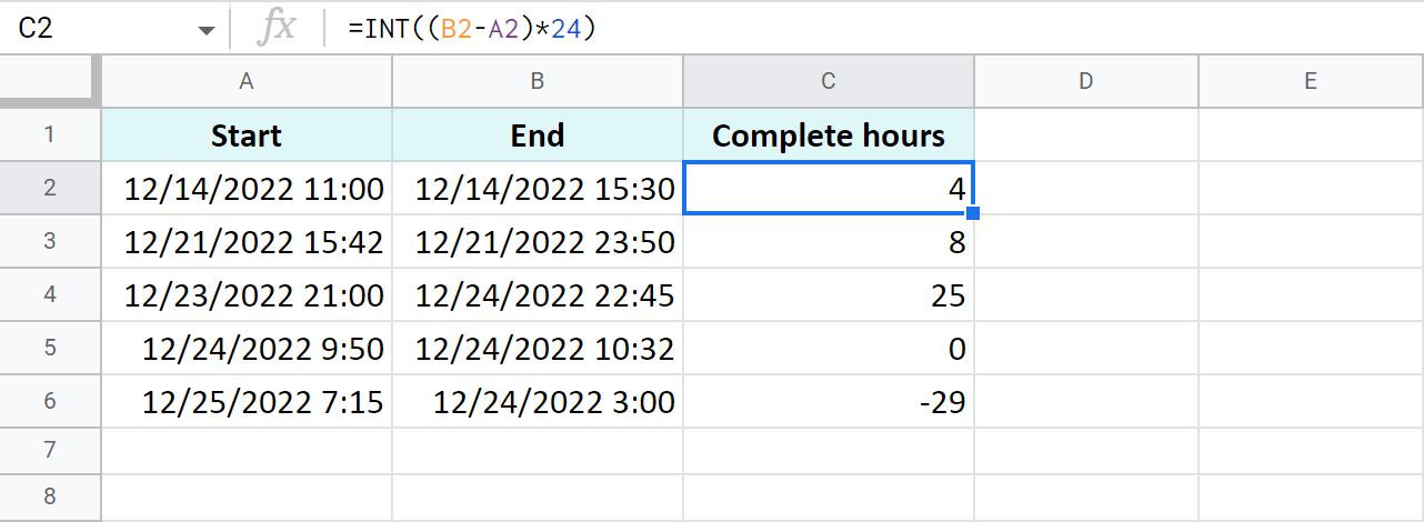
If the start time is greater than the end time, the formula will return a negative number, like in C5 in my example.
Tip. The INT function will let you see the number of complete hours spent since it rounds numbers down to the nearest integer:
-
To count minutes, subtract the start time from the end time and multiply whatever you get by 1,440 (since there are 1,440 minutes in one day):
=(End time - Start time) * 1440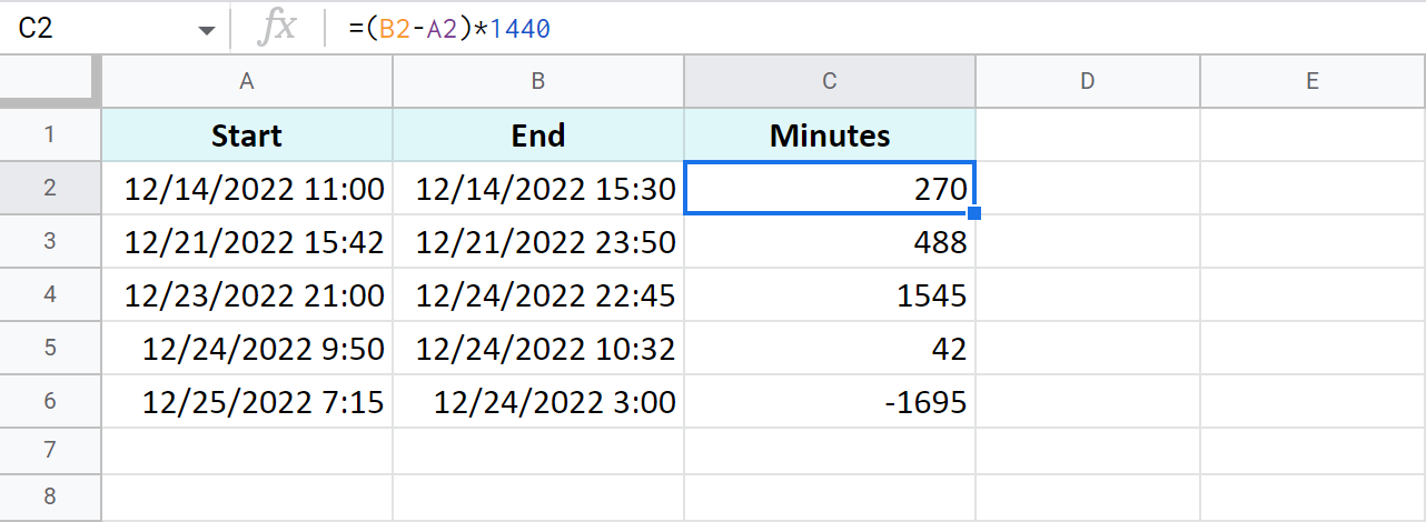
-
To find out how many seconds passed between two times, the drill is the same: subtract the start time from the end time and multiply the result by 86,400 (the number of seconds in a day):
=(End time - Start time) * 86400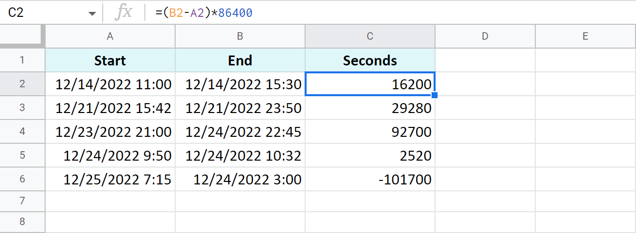
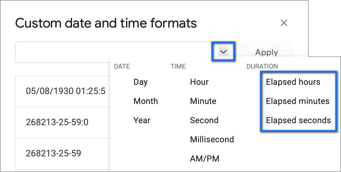
Tip. You can avoid multiplying in all these cases. Just subtract times first, and then apply elapsed time format from Format > Number > Custom date and time. If you click the down arrow to the right of the text field, you'll be able to choose between additional date and time units:
Example 4. Functions to get the time difference in a Google spreadsheet
As always, Google Sheets equips you with three particularly useful functions for this purpose.
Note. These functions work only within 24 hours and 60 minutes and seconds. If the time difference exceeds these limits, the formulas will return errors.
=HOUR(B2-A2)- to return hours only (without minutes and seconds)=MINUTE(B2-A2)- to return minutes only (without hours and seconds)=SECOND(B2-A2)- to return seconds only (without hours and minutes)

How to add and subtract time in Google Sheets: hours, minutes, or seconds
These operations can also be achieved with two techniques: one involves basic math calculations, another - functions. While the first way always works, the second one with functions works only when you add or subtract units less than 24 hours, or 60 minutes, or 60 seconds.
Add or subtract hours in Google Sheets
-
Add less than 24 hours:
=Start time + TIME(N hours, 0, 0)Here's how the formula looks on real data:
=A2+TIME(3,0,0)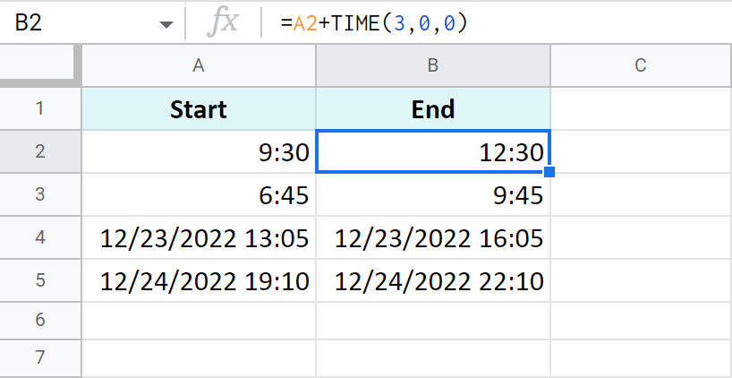
-
Add more than 24 hours:
=Start time + (N hours / 24)To add 27 hours to the time in A2, I use this formula:
=A2+(27/24)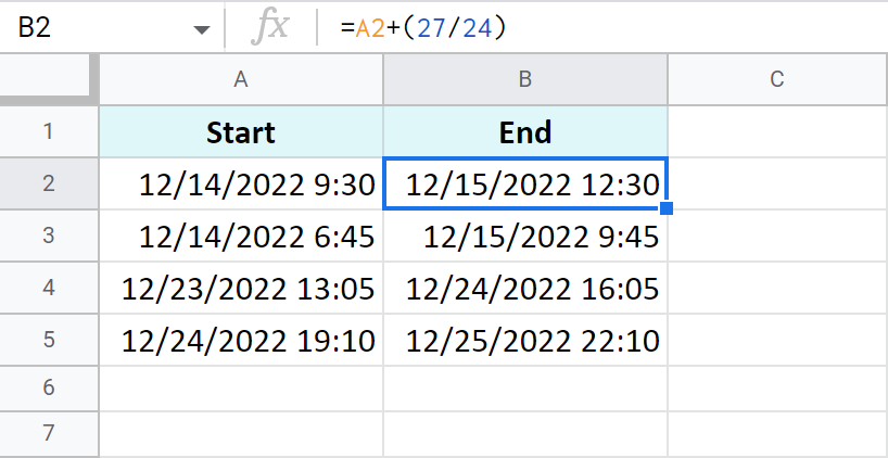
- To subtract 24 and more hours, use the formulas above as a basis but change the plus sign (+) to the minus sign (-). Here's what I've got:
=A2-TIME(3,0,0)- to subtract 3 hours=A2-(27/24)- to subtract 27 hours
Add or subtract minutes in Google Sheets
The principle of manipulating minutes is the same as with the hours.
-
There's the TIME function that adds and subtracts up to 60 minutes:
=Start time + TIME(0, N minutes, 0)If you are to add 40 minutes, you can do it like this:
=A2+TIME(0,40,0)If you are to subtract 20 minutes, here's the formula to use:
=A2-TIME(0,40,0)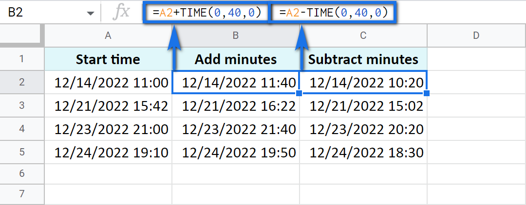
-
And there's a formula based on simple arithmetic to add and subtract over 60 minutes:
=Start time + (N minutes / 1440)Thus, here's how you add 120 minutes:
=A2+(120/1440)Put the minus instead of plus to subtract 120 minutes:
=A2-(120/1440)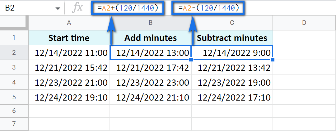
Add or subtract seconds in Google Sheets
Seconds in Google Sheets are calculated in the same manner as hours and minutes.
-
You can use the TIME function to add or subtract up to 60 seconds:
=Start time + TIME(0, 0, N seconds)For example, add 30 seconds:
=A2+TIME(0,0,30)Or subtract 30 seconds:
=A2-TIME(0,0,30) -
To calculate over 60 seconds, use simple maths:
=Start time + (N seconds / 86400)Add 700 seconds:
=A2+(700/86400)Or subtract 700 seconds:
=A2-(700/86400)
How to sum time in Google Sheets
To find the total time in your table in Google Sheets, you can use the SUM function. The trick here is to choose the correct format to display the result.
By default, the result will be formatted as Duration - hh:mm:ss
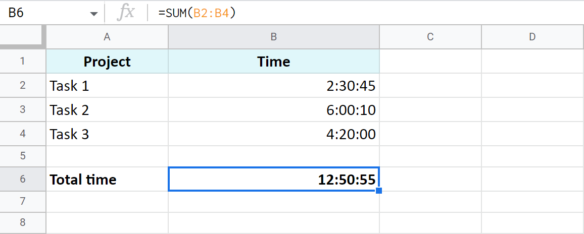
But most often the default time or duration format won't be enough, and you will need to come up with your own one.
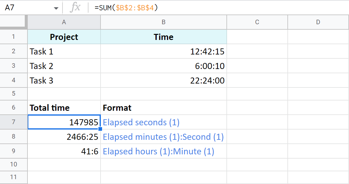
A7:A9 cells contain the same time value. They are just displayed differently. And you can actually perform calculations with them: subtract, sum, convert to decimal, etc.
Extract date and time from a full "date-time" record
Let's imagine that one cell in Google Sheets contains both, date and time. You want to set them apart: extract only the date to one cell and only time to another.
Split Date time using Number format
In order to display date or time in one cell on your screen or to print it, just select the original cell, go to Format > Number and choose Date or Time.
However, if you'd like to use these values for future calculations (subtract, sum, etc.), this won't be enough. If you don't see the time unit in a cell, it doesn't necessarily mean that it's absent, and vice versa.
So what do you do?
Split Date time using formulas
Google stores dates and time as numbers. For example, it sees the date 8/24/2017 11:40:03 as the number 42971,4861458. The integer part represents the date, the fractional - time. So, your task is down to separating integer from fractional.
- To extract date (integer part), use the ROUNDDOWN function in cell B2:
=ROUNDDOWN(A2,0)
The formula rounds the value down and casts the fractional part away.
-
To extract time, place the following subtraction formula into C2:
=A2-B2 -
Copy the results into the third row and apply Date format to B3 and Time format to C3:

Use the Split Date & Time add-on
You may be surprised but there's one special add-on for this job. It's really small and easy but its contribution to Google Sheets cannot be overstated.
Split Date & Time splits all Date time records in your entire column at once. You control the desired outcome with just 4 simple settings:
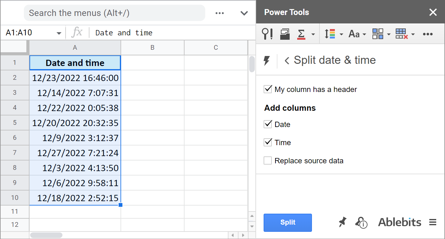
You tell the add-on:
- Whether there's a header row.
- If you want to get the Date unit.
- If you want to get the Time unit.
- And if you'd like to replace your original column with the new data.
It literally takes the burden of splitting date and time units off your shoulders:
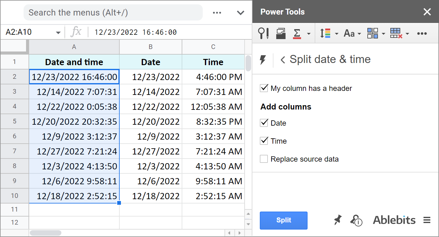
The add-on is part of the Power Tools collection so you will have more than 40 other useful add-ons at hand:
These are the ways to not only display date or time, but to separate them to different cells. And you can perform various calculations with these records now.
I hope these examples will help you solve your tasks when working with dates and time in Google Sheets.
Spreadsheet with formula examples
Calculating time in Google Sheets (make yourself a copy to practice)
 by
by 
379 comments
Great place to know more about advanced excel tricks and tips
I have a question let's suppose I want to add 2 hours to the time and date format columns and also want the date to change were adding 2 hours in the 24-hour clock make it the next day
example
Column A = Date + Time (02.11.2021 00:00:00)
Now by adding 2 hours in the above case date needs to be (03.11.2021 02:00:00)
Hello Amin,
I'm afraid the Google Sheets way of calculating this differs from your desired result. Since 02/11/2021 00:00:00 is midnight (the very beginning of 02/11/2021), adding 2 hours will result in 02/11/2021 02:00:00.
You need to have 02/11/2021 23:59:59 in order to switch to the next day with the calculation. Or simply add 26 hours instead: =A2+(26/24)
JJLIVERPOOL28 if you have anything to help help you help or help help me get
Hi!
Sorry, it's not quite clear what you are trying to achieve.
Hi Natalia, Can you please provide me simple formula in which I can calculate total hours they picked & packed in a day less the breaks they had. And also if they start for example picking around 2:00pm and they finished the next day around 11:AM. Our working hours starts at 7:30am until 4:00pm only. I hope you can help. Thanks.
Hi Cristine,
I'm sorry, I'm afraid these pieces of info are not enough to give you a formula. What about the breaks? Are they indicated in your document as well? Can they also start one day and end the next day?
For me to be able to help you better, please consider sharing a small sample spreadsheet with us (support@apps4gs.com) with 2 sheets: (1) a copy of your source data (2) the result you expect to get. I kindly ask you to shorten the tables to 10-20 rows.
Note. We keep that Google account for file sharing only and don't monitor its Inbox. Please do not email there. Once you share the file, just confirm by replying to this comment.
Hi,
I am trying to put a sheet that works out how many hours a team member has worked between 08:30 - 17:30 (weekdays) and how many hours they have worked outside of this on a shift (all day at weekends). The shifts can finish at any time including after midnight. I have tried multiple formulas with no success.
The cells that require attention are B27 to B36
The starting information is:
B27 = TIME(08,30,0) {start of in hour timeframe - fixed time}
B28 = TIME(17,30,0) {end of in hour timeframe - fixed time}
B29 = 00:00 {start time of shift - variable field}
B30 = F8+B29 {end time of shift - fixed value, F8 takes total shift time from another cell}
B32 = =IF((B30-F8)>TIME(6,30,0),TIME(6,30,0),"")
B33 = =IF(B30>TIME(17,30,0),IF(B30<TIME(23,59,59),B30-TIME(17,30,0),B32),0)
The most recent attempt at making this work came out as this:
B35 {out of hours worked} -
=(IF(B291,B30-1,0))-(if((if((B29+F8)>1,B30-1,0))>TIME(8,30,0),(if((B29+F8)>1,B30-1,0))-TIME(8,30,0),0)))+B33
B36 {in hours worked} -
=F8-B35
I have sent a copy of the template to yourselves (named "Work in progress"). I am aware that these calculations do not even begin to factor in the weekend shifts but wanted to establish the timings before moving onto when the date of the shift occurs.
Thank you for your guidance.
My apologies,
The formula in B35 is actually this:
=(IF(B291,B30-1,0))-(if((if((B29+F8)>1,B30-1,0))>TIME(8,30,0),(if((B29+F8)>1,B30-1,0))-TIME(8,30,0),0)))+B33
Hi Adam,
Thank you for sharing your spreadsheet and for the detailed description.
I'm afraid there are some moments that I don't understand in your tables. E.g. what those 6:30 hours mean in B32 and whether you'd like to take them into account for calculations as well. I'm also not sure what 'total premium time on shift' should contain. Is it different from B33?
I've adjusted your formula in B33 (my variant is in C33) as it looks like your formula contains odd 10 minutes.
For now, based on what I was able to understand, I would suggest to try using the following logic (see very simple demo cells on Sheet2):
How do. You subtract minutes from time?
Hello Abby,
Look for the title Add or subtract minutes in Google Sheets in this section. You will find formulas and a couple of examples there.
Hi Natalia,
I'm currently creating a work schedule for my new work place and im trying to convert induvial hours logged over 24hrs in one section into reading like a 24 hour clock in the another section of the schedule (eg 10.00 - 18.00) or if the person was off (libre) then "libre" would show up. Do you know if this is possible.
Thanks !
Hi Conor,
please consider sharing an editable copy of your spreadsheet with us (support@apps4gs.com) with 2 sheets: (1) your source data, (2) the result you expect to get. Please also shorten the tables to 10-20 rows.
Note. We keep that Google account for file sharing only and don’t monitor its Inbox. Please do not email there. Once you share the file, just confirm by replying to this comment.
If you have confidential information there, you can replace it with some irrelevant data, just keep the format. I’ll look into it and try to help.
Hi im trying to do Operators Efficency Sheet in Google Spreed Sheets i'v done most of it but hit dead end 2 weeks now
so the problem is on my sheet. differnce103800 in own column and in diffrent column i'v divied 200 gives me 519 and in diffrent column it's give me 8.65 it's not what im looking for im looking for 08:39:00 which is correct answer i'v tried everything can you help
please
Hi Matthew,
For me to be able to help you better, please share an editable copy of your spreadsheet with us (support@apps4gs.com) with 2 sheets: (1) a copy of your source data (2) the result you expect to get. I kindly ask you to shorten the tables to 10-20 rows.
Note. We keep that Google account for file sharing only and don't monitor its Inbox. Please do not email there. Once you share the file, just confirm by replying to this comment.
I'll look into it and try to help.
Hi I was wondering if there is a formula that can calculate the number of minutes after a specific time. I need total number of minutes after 3pm. Thank you!
Hi Kim,
Assuming your start time (3pm) is in A2, here's the formula to try:
=HOUR(NOW()-(TODAY()+A2))*60 + MINUTE(NOW()-(TODAY()+A2)) + SECOND(NOW()-(TODAY()+A2))/60
Make sure to format a cell with this formula as a number.
Hi there! I want to make a column that updates with a new number displayed every 6 hours. For example, it starts with 2, and after 6 hours have passed it displays 4 instead of 2. How would I go about this?
Hi Sara,
I'm afraid it's impossible with the standard Google Sheets features. You may try to find a solution here – an overview of Google Apps Script with a lot of helpful content and links: https://developers.google.com/apps-script/overview
Hi! My hope is that there is a sum formula for adding song lengths that contain hours, minutes, and seconds. I have them set up in this format: 01:04:35 but it doesn't add it as hours, minutes, and seconds... Is there a formula? Do I need to put each quantity in separate cells? hours in one, minutes in one, and seconds in another? thanks!!!!!
Hi Aimée,
If all of them are in the Duration format (01:04:35), you should be able to sum them correctly with a simple SUM function, please see the examples in this part of the article.
Is there a way when subtracting time to automatically convert time format of minutes to hours as my goal is like this:
On A1 is start time say 8:00 AM and on A2 is end time as 8:40AM, and it returns the duration on A3 as "40 mins".
What I aim is that if it's more than 60 mins, say A1 is 8:00AM and A2 is 9:20AM, it automatically formats A3 result to "1 hr 20 mins"
Hello John,
Try this formula:
=IF(MINUTE(A2-A1)>60, (HOUR(A2-A1)&" hours, "&MINUTE(A2-A1)&" minutes"), A2-A1)
i have to convert data in 3-3 hours conversion ex- if one message is popup on 12:00am then display 12:00am to 3:00am time slot, other message is came on 7:00pm then display 6:00pm to 9:00pm time slot
Hello Riken,
If I understand your task correctly, you need to use the IF function in your calculations.
Please could you help with the following? I am not sure what kind of formula should be used. I wanted to make use of a screenshot of an example of what I want, but it won't allow me to paste a screenshot.
I need to set up a program for a dancing competition. I have different sections in the dancing competition, with each section have different time limits per performer. So here is an example:
Section: Solo Start time: 9:00 AM
Competitor 1 (Maximum time: 3min:30sec) (Grace time: 2min)
Competitor 2 (Maximum time: 3min:30sec) (Grace time: 2min)
Competitor 3 (Maximum time: 3min:30sec) (Grace time: 2min)
Competitor 4 (Maximum time: 3min:30sec) (Grace time: 2min)
Competitor 5 (Maximum time: 3min:30sec) (Grace time: 2min)
(Grace time after each section: 2min)
End time: ?
Section: Improvisation Start time: SAME AS END TIME - ?
Competitor 1 (Maximum time: 2min:0sec) (Grace time: 1min)
Competitor 2 (Maximum time: 2min:0sec) (Grace time: 1min)
Competitor 3 (Maximum time: 2min:0sec) (Grace time: 1min)
So I want the condition to be, if it is a solo, then maximum time per competitor is 3min:30sec with 2min grace for each competitor, with 2min grace after section. Start time is 9AM, so what will the end time be after section has ended?
Hope the above example makes sense.
Thanks in advance
Hello Antoinette,
Feel free to share an editable copy of your spreadsheet with us (support@apps4gs.com) with 2 sheets: (1) a copy of your source data (2) the result you expect to get. I kindly ask you to shorten the tables to 10-20 rows. I'll look into it.
Note. We keep that Google account for file sharing only and don't monitor its Inbox. Please do not email there. Once you share the file, just confirm by replying to this comment.
Thanks so much Natalia. I have shared an editable sheet. It is just an example, as I cannot send the original sheet, because in our country there are laws against sharing people's information (especially children). I hope it makes sense. I do know what I want is quite complicated.
Thank you for sharing your spreadsheet, Antoinette.
I created a new sheet – Copy of the Result – and entered all formulas there. I use the IF function to return the times per competitors based on the section mentioned in A2. You can add more conditions for other sections with the help of nested IF or IFS to reuse the same formula for other sections as well.
The total duration is a simple sum of all those time units.
Hope this helps! Please let me know if this is what you need :)
Thanks so much for your help.
I was trying to make it very complicated, and it actually is not.
This really helped a lot.
Hope you enjoy your day.
You're most welcome, Antoinette!
Glad I could help :) Have a lovely day as well :)
Hey Natalia, hope you are well,
Just making sure you got my message on (May 20, 2022 at 5:14 pm)
Hi Jordan,
Sorry I couldn't reply earlier. I replied a few minutes back though, please see my comment below.
If you still need some help with your formulas, please consider checking out the blog post we wrote about the IF function. Or share your spreadsheet with us (support@apps4gs.com) with 2 sheets: (1) a copy of your source data (2) the result you expect to get. Please shorten the tables to 10-20 rows.
Note. We keep that Google account for file sharing only and don't monitor its Inbox. Please do not email there. Once you share the file, just confirm by replying to this comment.
Hi Natalia,
I have invited you to my Google Sheets for you, i think it would be the best way to figure it out.
Hi Jordan,
Thank you for sharing the file. Seeing the whole picture, we've come up with another solution. I entered the formulas on the Copy sheet, please take a look.
Hi Natalia,
I have been reading through your blog posts and they are really tremendous. Need your support on one of my on-going problems which I am trying to solve through formula in Google-Sheets :
1. end_date = Available = (Today())
2. Number of months = Available in decimal = (4.1) months
3. start_date = ? (how to compute it)
Your help in this would be much appreciated.
Best,
Deep
Hi Deep,
I'm sorry, I'm afraid I don't fully understand your task. Is that number of months shows the duration from the start time?
if I want to use =TEXT(B2-A2,"h:mm") to subtract time but I want it to display the result as 3h 2m how do I format it to do display it as such?
I ended up figuring it out after days of trying things it was super easy. This is for anyone interested.
Times:
D2 - 5:18:00 PM
E2 - 8:20:00 PM
=HOUR(E2-D2) & "h " & MINUTE(E2-D2) & "m"
Result - 3h 2m
Hi Victor,
Sorry I couldn't reply to you earlier. Happy to see you've got it figured out :) Thanks for sharing your solution!
I ran into an issue today where it won't subtract backwards times like pm to am. Such as
12:23 AM - 9:50 PM
It gives an error because it's a negative number and I still haven't found a workaround
Hi Victor,
The result I'm getting with this set of times is 21h 27m.
For me to be able to assist you better, please share a small sample spreadsheet with us (support@apps4gs.com) with 2 sheets: (1) a copy of your source data with the formulas that don't work (2) the result you expect to get. I kindly ask you to shorten the tables to 10-20 rows.
Note. We keep that Google account for file sharing only and don't monitor its Inbox. Please do not email there. Once you share the file, just confirm by replying to this comment.
Yes but that result is backwards and not correct. 12:23 Am is right after midnight. If you subtract midnight to 9PM that is only 3 hours we are trying to subtract not add.
I'm building a sheet to track all of my forex trading. I want to enter the time I start a trade and the time I end a trade and it tell me how long that trade went for. So I can keep an idea on how long these trades are lasting. Yesterday I started a trade at 9:50 PM and it went until 12:23 AM which is right after midnight. So I need it to subtract the time.
The result I'm looking for is 2h 33m
Thank you for the update, Victor.
If you enter time without a date, Google Sheets treats these times as from the same day. You can check that by changing the format to Date time.
So I'd advise you to enter both date and time to your cells (just set the format as Time to keep the date hidden) and you should get the correct results.
Can you give me a sample sheet that I can take a look at. I'm currently using two cells to collect this data. One for just the date and one for just the time.
4 cells total. Date, Time Start, Time End, Time completed
Hello Victor,
If you'd like to take a look at how the formats work, you will still need to go to the Format settings to see the difference. So you can just literally (1) enter 9:50 PM into one cell and both, time & date, e.g. 06/02/2022 9:00 PM, in another, (2) select both these cells, (3) and go to Format > Number a few times and try to apply different formats, including those with the date unit. You'll instantly see what I mean about the dates.
For me to be able to help you better, I kindly ask you to share your sample sheet with us: support@apps4gs.com. You don't need to provide your entire document. A sheet with a few rows showing your source data and a sheet with the result you expect to get is more than enough. Thank you.
We need formula for if working hours is 6 and 1 person working 6.5 hours and we need to show he worked 0.5 hour extra (fixed time 10:00AM to 04:00PM) (Work time 10:00 AM to 4:30:00PM) actual extra work 0.5 hour
what is the formula for that
Hello Balajinaik,
You need to use the IF function for such calculations:
=IF((B2-A2)*24>6,(B2-A2-TIME(6,0,0))*24,"")
Hello Natalia,
I use google sheets to do wages and I need a bit of help to sort an issue.
Regular work hours are 9am to 6pm (important to remember) and I'm trying to subtract overtime hours or minutes that my employees work.
For example, Start time is (7am) and the finish time is (9pm), I'd then like it to separate in another cell the 2 overtime hours from the starting point (7am-9am) and the 3 overtime hours from the finish point (6pm-9pm)
Look forward to hearing back from you.
Hello Jordan,
Assuming your start time is in A2 and end time is in B2, try these IF formulas in C2 and D2:
=IFS(OR(A2<TIME(9,0,0),A2>TIME(9,0,0)),TIME(9,0,0)-A2,A2=TIME(9,0,0),"")
=IFS(OR(B2>TIME(18,0,0),B2<TIME(18,0,0)),B2-TIME(18,0,0),B2=TIME(18,0,0),"")
Hey Natalia, thank you for getting back to me.
So far the C2 format is working and I'm assuming that you missed out a comma in this area [A2TIME] but I have replaced it with [A2,TIME] and it's working.
For the D2 format, I am getting an error message, see the error message below.
[Wrong number of arguments to IFS. Expected at least 2 arguments, but received 1 arguments.]
I have also just noticed, that when I add the start time 10am. In C2 I get [23:00:00]. Is there any way to make it 00:00:00 if the start time was anytime after 9am?
At the moment, the formulas calculate the negative number if the start time is after 9am. But if you'd rather see 00:00:00, then you need to write out each condition and the required result in the formula:
=IFS(A2<TIME(9,0,0),TIME(9,0,0)-A2,A2=TIME(9,0,0),"",A2>TIME(9,0,0),TIME(0,0,0))
Thank you ever so much for the help you have provided so far.
This format:
=IFS(A2TIME(9,0,0),TIME(0,0,0))
What would the format be for a time before 6pm?
You're most welcome, Jordan :)
As for time before 6pm – if you'd like to add a condition for when the start time is before 6, just add the same part you quoted to the formula but change 9 to 6. If you mean you'd like to add conditions for the end time as well, please specify what you'd like to return if it's before/after/equals 6.
Hiya Natalia,
I'm not sure what I even wrote in the last reply, I'm confused myself lol.
So at the moment with the new [FORMAT] you provided, whenever I type anything after 9am it says 00:00:00 which is correct and id now like another format to do the same for when I write a time that is before 18:00:00 it should say 00:00:00 and it would only count the time after 18:00:00.
[FORMAT] you provided earlier:
=IFS(A2TIME(9,0,0),TIME(0,0,0))
Another note, not a huge issue, so when using the [FORMAT] and typing a time for example 10:00:00, it says 00:00:00. Is it possible to just have it blank using the '' ''?
I can see the confusion now, I'm trying to type the full [FORMAT] in the reply but for some reason it changed and doesn't post the hole thing?
Hopefully this works, this is what I'm trying to type:
=???(??????(?,?,?),????(?,?,?))
Its done it again, let me try another font:
[=̶I̶F̶S̶(̶A̶2̶̶T̶I̶M̶E̶(̶9̶,̶0̶,̶0̶)̶,̶T̶I̶M̶E̶(̶0̶,̶0̶,̶0̶)̶)̶]
I am trying to type the format you sent me on (May 19, 2022 at 6:49 am) Spain time.
Hi Jordan,
For when the time is before 18, the drill is the same: you need to put that as a pair of "condition, it result" in the formula. Just like I did with 9, but only with 18 this time:
=IFS(A2<TIME(18,0,0),TIME(0,0,0),...)
If you prefer empty cells rather than 00:00, yes, feel free to use "" instead.
=IFS(A2<TIME(18,0,0),TIME(0,0,0),...)
Btw, I still suggest you look through this blog post about the IF function :) You just may find the answers to your questions there much faster than I can reply :)
Hi Jordan,
My apologies, the formulas appeared broken due to > and < symbols. I've edited the formulas, please take a look now.
I typed a start time colum and an end time colum via the 13:25 format (the date is on a separate colum): I don't understand how to calculate the subtraction : meaning the differnce between them.
How can I do that please?
Hello Sharon,
You need to subtract end time from start time. Please see the examples here:
Example 1. Subtract time to get the time duration in Google Sheets
Hello - trying to get google sheets to auto calculate clock out time for me - IE i put in / out time in for monday- thursday, and only in time on friday. Id like google to do the math for the final clock out, except it giving me negative total hours and the rest of the numbers dont seem to jive....
Hello Vernon,
For me to be able to help you, please share an editable copy of your spreadsheet along with your formula with us: support@apps4gs.com. I'll look into it.
Note. We keep that Google account for file sharing only and don't monitor its Inbox. Please do not email there. Once you share the file, just confirm by replying to this comment.
sent the link via gmail
Thank you for the example, Vernon.
Your formula doesn't work because you use 40 as an integer, not as a number of hours. I've entered the correct formula to F6:
=B6+(TIME(40,0,0)-SUM(D2,D3,D4,D5))
I have a number which is 16.80
so since there is no 0.80 in minutes, it has to be converted to 0.70+0.20 so time becomes 17.20
Want to represent the time as 17.20
How do I do this
Hello Asha,
Try this formula:
=IF(INT(A1)=A1,A1,ABS(0.6-(A1-INT(A1)))+CEILING(A1))
I'm having an issue where the formula =(f2-e2,"h:mm") is returning times that are off by a minute. For example cell e2 is 01:18 and cell f2 is 03:38. The above formula completes as 02:19 when it should be 02:20. This is happening on a significant portion of data I am trying to create.
Hello Jason,
You formula doesn't work on my side at all (formula parse error). However a simple =F2-E2 returns 02:20.
For me to be able to help you, please share an editable copy of your spreadsheet with the formula that returns 02:19 with me: support@apps4gs.com. I'll look into it.
=E10-D10+G10-F10+I10-H10+K10-J10+M10-L10+O10-N10+Q10-P10
I am trying to calculate wages and I need the spreadsheet to multiply hourly pay by hour worked for multiple employees. Specifically I need a specific cell to multiply and add 6 cells together across 3 rows and it is returning decimal numbers and that cell is affecting another cell i have that is supposed to divide that information with another cell and because i am getting decimal numbers it is throwing off the end result that i am looking for.
Hello Adam,
I'm sorry but your question is not clear.
For me to be able to help you, please share a small sample spreadsheet with me (support@apps4gs.com) with 2 sheets: (1) a copy of your source data (2) the result you expect to get (the result sheet is of great importance and often gives us a better understanding than any text description). I kindly ask you to shorten the tables to 10-20 rows.
Note. We keep that Google account for file sharing only and don't monitor its Inbox. Please do not email there. Once you share the file, just confirm by replying to this comment.
Thank you.
Hi, I have a sheet to work out staff hours and when time worked is over 24 hours for example 33:20:00 the formula i use to covnert this into a decimal amount of hours does not work and give me the amount of hours worked over 24 hours. I am using this formula below:
=(HOUR(E59)+MINUTE(E59)/70+SECOND(E59)/3600). I have tried changing the data type of the cell to [hh]:mm:ss but this still doesnt work. Do you have any suggestions?
Thank you!
Hi Declan,
33:20:00 already shows the duration of hours (33). You can either multiply this by 24 (see Example 3. Time difference in hours, minutes, and seconds; make sure the resulting cell is formatted as Number) or change the time format into elapsed hours only.
Hi, thank you for this info.
Just FYI, I think there is a typo in the extract the date/time section. Formula 2, says A2=B2, and I to match the image, it should say A2-B2.
Hi Natalia,
Thank you for your feedback!
That is definitely a typo. I've just corrected it, thanks a lot! :)
Hello,
How would I check to see if a time is within a time range when the range goes past midnight? (i.e: The time to check is 03:00 and the time range is (21:00 - 5:00). Any help will be appreciated, thanks!
Hello Jay,
Is your time range in one cell or each time unit is in its own cell?
Hello Natalia,
The range is in one cell (i.e 5:00pm - 5:00am). I can parse out the separate times, but I can't get it to realize that a time (i.e 3:00am) is in between the range since the time value is lower than the beginning of the range.
If it makes it easier to have each time in it's own cell, I can create helper columns (split) to separate them.
Hello Jay,
Assuming that 3:00am is in A2, 5:00pm – in B2, and 5:00am – in C2, the following formula will return TRUE if the time falls within the range, otherwise, you'll see FALSE:
=OR(AND(B2>A2,C2>A2),AND(B2>A2,C2>A2))
Hi Natalia, I'm sorry if this has already been asked/answered. I wondered if there was a way to add 2 seconds to a time formatted in a 00:00:00 AM/PM format. Ex( start time is 10:05:03 AM, and I want the end time to be 10:05:05 AM) I am trying to get a formula to add markers for video/audio edits quickly. This has been rattling around in my head for a while now, and I can't seem to figure it out! I would be super grateful if you knew how to accomplish this!
Hi Leah,
Have you tried ways from 'Add or subtract seconds in Google Sheets' in this section of the blog post?
Hello! I am having difficulty doing a duration countdown. I have cells with a date & time something is due (call it A1) and another cell with the NOW() function in it (call it B1) , those both work. When I do B1-A1 it returns a duration which counts down, however it's not the correct time. I read that google uses a different reference year and add a +1 at the end which worked for some, but as they get closer to less than 24 hours they then add 31 days on the front. For one that has 17 hours 33 mins remaining it states 31 days 17 hours 33 mins remaining.
Any ideas?
best,
mattkwi
Hello mattkwi,
Can you please specify the exact date time from A1 and the result your B1-A1 returns so I could understand your case better?
Hello, I'm trying to fix so that i can have name down in A, Times in minutes, seconds, and milliseconds in B, and the difference between them in C
Example
A B C
Name Time Difference
Rodney 1m:25s:754ms 0.000
Peter 1m:26s:516ms ??????
please help! :D Thank you :D
Hello Torbjørn,
First, you need to enter your durations in the correct format so Google Sheets could treat the contents as Duration:
Then you'll be able to calculate the difference between them.
Is it possible in Google Sheets to subtract 2 durations that are not linked to an AM/PM time? I am a swimming coach and I am hoping to use Sheets to calculate the difference between two race times. For example, I have a swimmer who swims the 50 yard butterfly. Her current time is 1:05.39 (mm, ss , ms) and her goal time is 35.83 (mm, ss, ms). Is there a formula I can use for this? One of the challenges is that I am subtracting different values (minutes and seconds capping out at 60 and then converting, milliseconds going all the way up to 100 before converting)
Thanks for any feedback or guidance you can give!
Hello Else-Marie,
For Google Sheets to understand the exact format of the entered values, try the following:
Then try calculate these durations, it should work.
Hi, I am also a coach that uses race times. I am having a very hard time as well.
I have many athletes that have times in (mm, ss , ms) ONLY.
I tried to use the format of hh:mm:ss.000 however it calculates to a 24 hour model. I am not using any hours at all in my splits for racing.
I need something like this
Athelte A- 1:04.75
Goal time- 1:03.09
I need the differences so it would be -1.66 so that my athlete knows that they need to drop 1 seconds and 66 mil seconds.
Thanks for all your help
Hi Andrew,
If setting the custom number format doesn't work for you, try the custom date and time format instead with the following:
Elapsed minutes (01):Elapsed seconds (01).Miliseconds (01)
Make sure to apply the same format to the resulting cells.
Hi,
I think I read most of the comments and unfortunately I cannot find a solution to my problem.
I need to add 52 hours to a date (08/11/2021 12:02:36) my problem is that I want to exclude the weekends.
In this case A1 = start date and my formula is =A1+time(52,0,0), I tried using =WORKDAY.INTL but it doesn't work.
Any help would be great and I love the your work.
Hi Vytaute,
Your formula to add 52 hours is incorrect. Here I mention the correct way (how to add more than 24 hours).
And here's a formula to add those 52 hours ignoring the weekends:
=IF(OR(WEEKDAY(A1+(52/24))=1,WEEKDAY(A1+(52/24))=7),IF(WEEKDAY(A1+(52/24))=1,A1+DAY(1)+(52/24),A1+DAY(2)+(52/24)),A1+(52/24))
It adds 52 hours first and checks if the resulting date is Saturday or Sunday. If so, it adds 2 or 1 day correspondingly.
Is it possible to calculate elapsed time in Sheets using a defined start date/time, and the CURRENT date/time as the end point? For example, if I specified a start date and time, is there a way for it to output the number of days, or preferably hours that have elapsed since then?
Hi BJ,
You can use NOW() and TODAY() functions instead of the specified end date/time, but these functions are volatile meaning they update themselves each time you open the spreadsheet or make edits anywhere in the file. Hence, your result will constantly update based on today's date/time.
But you can also use these functions to get the required results first and then turn them into values to stop further recalculations.
I am banging my head about this. I have a daily datetime stamps of a typical day at work starting at "10/22/2021 08:30:00 A" and ending at "10/22/2021 04:15:00 P". How can I filter out employees based on certain times of the day? Say 7 out of 10 employees start at 10/22/2021 12:15:00 P and end at 10/22/2021 03:15:00 P. How can I filter out those employees?
Any help is greatly appreciated.
Hello Alex,
If I understand your task correctly, you can (1) filter the rows (hide those that doesn't match your criteria); (2) or count the number of employees; (3) or even pull the required employees to a separate table.
Hi! I've used the following formula to find the duration of daily writing sprints:
=IF(INT(E3-D3)>0, INT(E3-D3) & " days, ","") & IF(HOUR(E3-D3)>0, HOUR(E3-D3) & " hour(s), ","") & IF(MINUTE(E3-D3)>0, MINUTE(E3-D3) & " minutes ","") & IF(SECOND(E3-D3)>0, SECOND(E3-D3) & " seconds","")
Now I want the sum of the duration times to find the total for the week. How can I do this?
Once I do that, I'd like to sum across multiple pages/sheets within the document so I can find the total for the month. Is this possible?
Hi Liz,
For me to be able to help you better, please share a small sample spreadsheet with us (support@apps4gs.com) with 2 sheets: (1) a copy of your source data (2) the result you expect to get. The result sheet is of great importance and often gives a better understanding than any text description. I kindly ask you to shorten the tables to 10-20 rows. I'll look into it.
Note. We keep that Google account for file sharing only, please do not email there. Once you share the file, just confirm by replying to this comment. I'll look into it.
I have shared my spreadsheet example with you as requested.
Hi Liz,
I'm sorry for the delay in my reply, I was on sick leave. Please let me know if you're still looking for a solution, I'll look into your file then.
You must get over 800 things
Hi,
I've got a starting date and a number of shift, If i sum the starting date and the shift it will find a delviery date, but I would love to avoid Holidays and week ends.
Could you help me?
Hi Federico,
You need to use the NETWORKDAYS function. You will find instructions and usage examples in this blog post.
Hi, is there a way to make it so it can calculate the time between two time frames if they're in the same cell?
i.e
8:00-13:00
Hi Ryan,
Yes, RIGHT & LEFT + SEARCH will help you out:
=RIGHT(A2, SEARCH("-", A2))-LEFT(A2, SEARCH("-", A2)-1)
Don't forget to apply the Duration format to the result.
Thank you so much! I was starting to think that excel has skipped this part!!
Hi,
These are instructions for Google Sheets :) Note that Excel functions may have different arguments.
hey, I was just wondering how to calculate elapsed time from velocity and distance in google sheets.
Hello Tom,
Could you please provide a couple of examples of your source records and of the result you'd like to get?
Hi!
This is article is pretty helpful. Do you have any idea of how to calculate time within/outside of business hours? For instance, if Column A's data is 1/1/2021 5:20AM and Column B's data is 1/6/2021 2:30PM, I'd like the total time elapsed minus the time we're unavailable (I can provide the business hours - but in this example let's say we're completely closed Sat/Sun and are open from 10am-5pm Mon-Friday)?
Any help would be greatly appreciated.
Thanks
Hi AC,
Thanks for stopping by our blog! :)
Assuming your start time is in A2, end time – in B2, opening time – F2, closing time – G2, the following formula will do the trick:
=(NETWORKDAYS(A2,B2)-1)*($G$2-$F$2)+MOD(B2,1)-MOD(A2,1)
If there are any special holidays you'd like to take into account, you can set them right in the NETWORKDAYS function. You'll find a tutorial about it in this blog post.
Hi! First I absolutely love this post and all of your kind responses. This has been so helpful to me.
Second, I am trying to work out a formula I am hoping you can help with. I want a formula to calculate the duration of time (in decimal form such as 1.25 for an hour and 15 minutes) if the time start/end is entered manually. I can do this perfectly using your above suggestions IF I ENTER THE TIME IN MILITARY TIME ONLY.
I want this to calculate the exact same way by being able to enter the time as you normally such as start at 11:00 and end at 2:00 without it resulting in a negative number. Is there any way to do this?
THANK YOU SO MUCH IN ADVANCE!
Hi Cait,
Appreciate your lovely feedback!
I described how to calculate the time difference in decimals in the 3rd example here.
However, if you use timestamps like this: start at 11:00 and end at 02:00, your spreadsheet won't understand that they belong to different days. You need to add days as well (19/08/2021 02:00:00) and then format cells to display the timestamp only. Then the time difference will be calculated correctly (a positive number).
Can I insert Live Countdown in Google Sheets?
Hello Rezu,
Yes, but we don't have a tutorial on our website. If you Google a bit, you'll find plenty of instructions, even demo videos, along with templates to use.
In my Spreadsheet, Whenever I input a data in a row Timestamp is auto added in this format 8/17/2021 20.05.31. I want that a countdown of 48 hours from the inputted Date and time. Can you help me? What would be the formula for subtracting 48 hour from the timestamp?
Hello Rezu,
I described how to subtract more than 24 hours in this part of the article, please have a look.
Hello there!
I´m trying to figure out how to get a timespan from a list of dates/times but cant seem to figure it out.
For example:
10/06/2020 19:28:55
15/06/2020 02:39:43
15/06/2020 06:30:04
16/06/2020 23:50:49
I want to see the elapsed timeframe between these different times.
10/06/2020 19:28:55 - 4 days, 5 hours, 10 minutes, 52 seconds till below time
15/06/2020 02:39:43 - 0 days, 3 hours, 50 minutes, 21 seconds, etc....
15/06/2020 06:30:04 - etc.etc.
Anyone know if this is possible and how i can make this appliable to a long list of dates and times?
Hello Niklas,
Try a formula like this:
=INT(J4-J3)&" days "&TEXT(J4-J3,"h"" hours ""m"" minutes ""s"" seconds""")
how can I get the "days" to just show up as 24 hours - for example,
Start time: 09/21/2022 08:00:00
End time 09/22/2022 13:00:00 with formula =INT(J4-J3)&" days "&TEXT(J4-J3,"h"" hours ""m"" minutes ""s"" seconds""") it would display 1 days 5 hours 00 minutes 00 seconds....
how can it show results as: 29 hours 00 minutes 00 seconds?
Hello Claudia,
try to simply subtract times (e.g. B2-A2) first and then apply the custom number format. See the very last tip in the Example 3 in this section.
Good night!
My goal is to add up all the hours worked in a month in a single cell.
That is, if I work:
07/04: 4:30 hours
5/07: 9 hours
06/07: 15 hours
07/10: 8 hours
07/15: 3 hours
07/20: 16 hours
I would like to get a cell that sums everything (= 55:30 hours)
I have tried with SUM and changing the format to "hours elapsed: minutes elapsed" or "hours: minutes" but I get absurd results (for example 2:30 or 26, never 55 and a half hours)
Is there a simple way to solve this? The fewer cells you use, the better.
Ok, I found the reason why SUMA was not working for me.
In the working range from 18h to 24h, the "24" interprets it as 00: 00h but NOT the 00: 00h at the end of the day and yes as 00: 00h at the beginning of the day (that is, -18 hours instead of +6 hours)
I managed to change that and it already works fine for me.
hello,
how you solved it ?
what is formula of this problem ?
please tell me
Hi!
I am trying to use a formula to determine hours worked in decimal form when we have shifts that often go past 12am. I need a way to do this where the outcome is not negative and can be all done in one formula, is that possible?
For example:
I have tried using both:
=TEXT(B2-A2, "h.m")-0.3 to try and get hours worked minus break time but this will not convert to decimal
= ((B2-A2)*24)-0.5 but this one causes negative numbers for any shifts that go past 12am
Hi Alexa,
You can turn negative numbers into positive by embedding your formula into the ABS function.
If this still doesn't solve your task, please consider sharing a short sample table with us – support@apps4gs.com. I'll look into it.
Note. We keep that Google account for file sharing only and don't monitor its Inbox. Please do not email there. Once you share the file, just confirm by replying to this comment.
hi can anyone help
How To Convert Time To Decimal Over 24 Hours In Google sheet?
=HOUR(A1)+MINUTE(A1)/60
Hi Zalmen,
I mention decimals in the following section: "Example 3. Time difference in hours, minutes, and seconds.". It's in the first part of the blog post, please take a look.
Also, here are some comments where I suggested formulas: Also, here are some comments where I suggested formulas: SUM and convert to decimal, format values correctly to see decimals.
If you're still unable to get the result, please specify (1) the exact time value you're trying to convert, (2) the formula you're using (3) and the result you're getting. I'll do my best to help.
Hello,
I am trying to create a google chart that automatically populates the 24 hour mark from the date and time I input in column A.
Example:
A
6/17/2021 8:09 pm
B- will automatically populate the date and time 24 hours later
6/19/2021 8:09 pm
Please assist
Hello Kim,
Just make sure the Data range that is used by the chart includes all cells (even empty ones) that will be filled in future. For example, B2:B100. Once they are filled, they will be shown in the chart as well.
If that's not really the problem, consider sharing an editable copy of your spreadsheet with us (support@apps4gs.com).
Note. We keep that Google account for file sharing only and don't monitor its Inbox. Please do not email there. Once you share the file, just confirm by replying to this comment.
I'll look into it and try my best to help.
if I want to multiply time?
For example I have a base time of 0:08 minutes and I want to multiply it by for eaxmple "10", in which the result would be 1:20 hours?
I've tried =0:08*10 but it gives me #ERROR!
What should I do?
Hello Mike,
You're getting the error because when you enter =0:08*10 that 0:08 is treated as text. This happens because Google Sheets doesn't see date and time the same way you see them. Please read about it here.
For the calculation to work correctly, I'd advise you to enter 0:08 in a separate cell. This will let Google Sheets recognize the record (you'll see that the format in a cell will change to 00:08 while the formula bar will show 00:08:00). Then reference this cell in a formula from another cell: =A2*10
Or use a formula like this: =TIME(0,8,0)*10
Hi Natalia,
First of all, thank you for the amazing article and responses in the comments!
I'm evaluating the time it takes to do certain tasks, and I was able to build a table with the correct duration values. This table includes values over 24 hours of duration, for example, "25:04:00".
In the table, everything works great, the conditional formatting for values over 24 hours works, and everything is perfect. However, I created a chart from this table, and the chart doesn't work as well.
It's a combo chart with bars representing the duration over time, and lines to represent the objectives and targets. Taking the example above, instead of 25 hours, the bar represents only 1 hour. It resets at 24 hours.
Even worse, another chart that is a copy of the first but feeds on different values, will reset values at 12 hours.
I can't seem to find any setting to control this. Can you help me?
Hi Tari,
Appreciate your kind feedback :)
For me to be able to help you with the chart, please share an editable copy of your spreadsheet with your table and the chart with us (support@apps4gs.com). If you have confidential information there, you can replace it with some irrelevant data, just keep the formats and durations intact.
Note. We keep that Google account for file sharing only, please do not email there. Once you share the file, just confirm by replying to this comment. I'll look into it.
I'm trying to tally up 2 different columns of times and determine the difference between them. Both sets of columns have an end time, subtracted by the start time to determine duration. I have the result of the formula formatted as "[h]:mm." Most of the time, the value is positive, more time was spent rather than what was estimated. However, there are some times when the actual hours worked were less than what was expected. I'm trying to keep a running tally of hours 'owed' as opposed to extra.
I am working on an old computer with an old version of Excel. It doesn't have as many of the formatting possibilities as you have listed in your examples above. The formula works when it returns a positive time duration, but the negative time is expressed as "####" because it says that there is no 'negative' time? Is there a workaround for this? Do I need to convert the time value to "real" numbers, keep a running sum, then put them back into time format for a total number of hours minutes? Could I incorporate an if/then statement?
I'm not as familiar with Goggle Sheets. I am going to be sharing this data with someone via Sheets and if there is a better/easier way to use it directly I can just avoid Excel altogether.
Thanks for your "time!" ;)
Hello Susan,
The instructions in this blog post are for Google Sheets. For Excel, you will find them in this article. There Svetlana mentioned how to make Excel display negative time. Hope this helps!
But if you're okay working with Google Sheets, there's only one version of Sheets and it shows negative time by default. Feel free to calculate everything in Google Sheets and let me know if it doesn't work as you expect there.