Whether there's summer knocking on our doors or winter invading Westeros, we still work in Google Sheets and have to compare different pieces of tables with one another. In this article, I'm sharing ways of matching your data and giving away tips on doing that swiftly.
Compare two columns or sheets
One of the tasks you may have is to scan two columns or sheets for matches or differences and identify them somewhere outside the tables.
Compare two columns in Google Sheets for matches and differences
I'll start by comparing two cells in Google Sheets. This way lets you scan entire columns row by row.
Example 1. Google Sheets – compare two cells
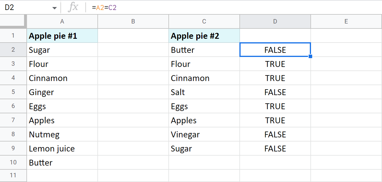
For this first example, you will need a helper column in order to enter the formula into the first row of the data to compare:
=A2=C2
If cells match, you'll see TRUE, otherwise FALSE. To check all cells in a column, copy the formula down to other rows:
Tip. To compare columns from different files, you need to use the IMPORTRANGE function:
=A2=IMPORTRANGE("spreadsheet_url","Sheet1!A2")
Example 2. Google Sheets – compare two lists for matches and differences
- A neater solution would be to use the IF function. You'll be able to set the exact status for identical and different cells:
=IF(A2=C2,"Match","Differ")
Tip. If your data is written in different cases and you'd like to consider such words as different, here's the formula for you:
=IF(EXACT(A2,C2),"Match","Differ")Where EXACT considers the case and looks for the complete identicals.
- To identify only rows with duplicate cells, use this formula:
=IF(A2=C2,"Match","") - To mark only rows with unique records between cells in two columns, take this one:
=IF(A2=C2,"","Differ")
Example 3. Compare two columns in Google Sheets
-
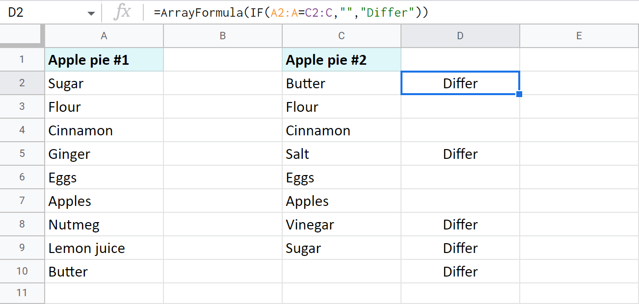
There's a way to avoid copying the formula over each row. You can forge an array IF formula in the first cell of your helper column:
=ArrayFormula(IF(A2:A=C2:C,"","Differ"))This IF pairs each cell of column A with the same row in column C. If records are different, the row will be identified accordingly. What is nice about this array formula is that it automatically marks each and every row at once:
-
In case you'd rather name the rows with identical cells, fill the second argument of the formula instead of the third one:
=ArrayFormula(IF(A2:A=C2:C,"Match",""))
Example 4. Compare two Google Sheets for differences
Oftentimes you need to compare two columns in Google Sheets that belong inside a huge table. Or they can be entirely different sheets like reports, price lists, working shifts per month, etc. Then, I believe, you can't afford to create a helper column or it can be quite difficult to manage.
If this sounds familiar, don't worry, you can still mark the differences on another sheet.
Here are two tables with products and their prices. I want to locate all cells with different contents between these tables:
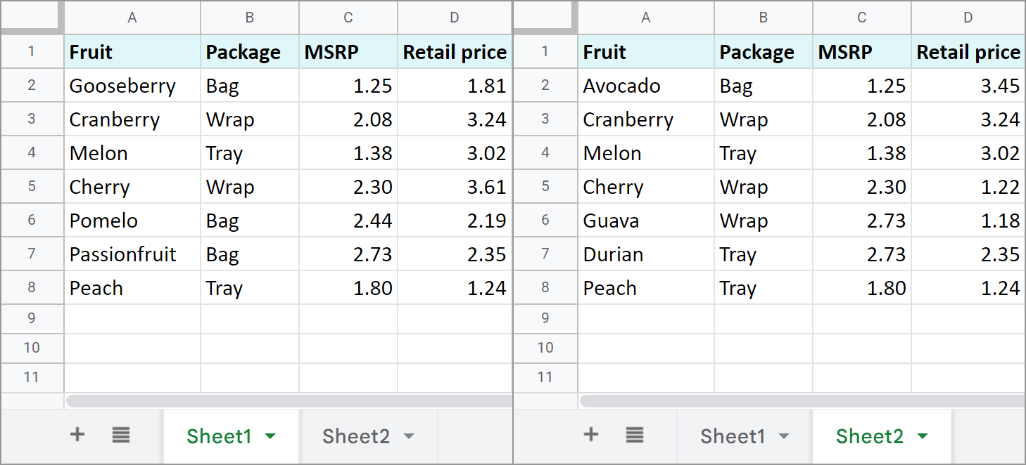
Start with creating a new sheet and enter the next formula into A1:
=IF(Sheet1!A1<>Sheet2!A1,Sheet1!A1&" | "&Sheet2!A1,"")
Note. You must copy the formula over the range equal to the size of the biggest table.
As a result, you will see only those cells that differ in contents. The formula will also pull records from both tables and separate them with a character you enter into the formula:

Tip. If the sheets to compare are in different files, again, just incorporate the IMPORTRANGE function:
=IF(Sheet1!A1<>IMPORTRANGE("2nd_spreadsheet_url","Sheet1!A1"),Sheet1!A1&" | "&IMPORTRANGE("2nd_spreadsheet_url","Sheet1!A1"),"")
Tools for Google Sheets to compare two columns and sheets
Of course, each of the above examples can be used to compare two columns from one or two tables or even match sheets. However, there are a few tools we created for this task that will benefit you a lot.
Compare sheets add-on for Google Sheets
This first one will compare two (& more!) Google sheets and columns for duplicates or uniques in 5 steps. Make it mark the found records with a status column (that can be filtered, by the way) or color, copy or move them to another location, or even clear cells and delete entire rows with dupes whatsoever.
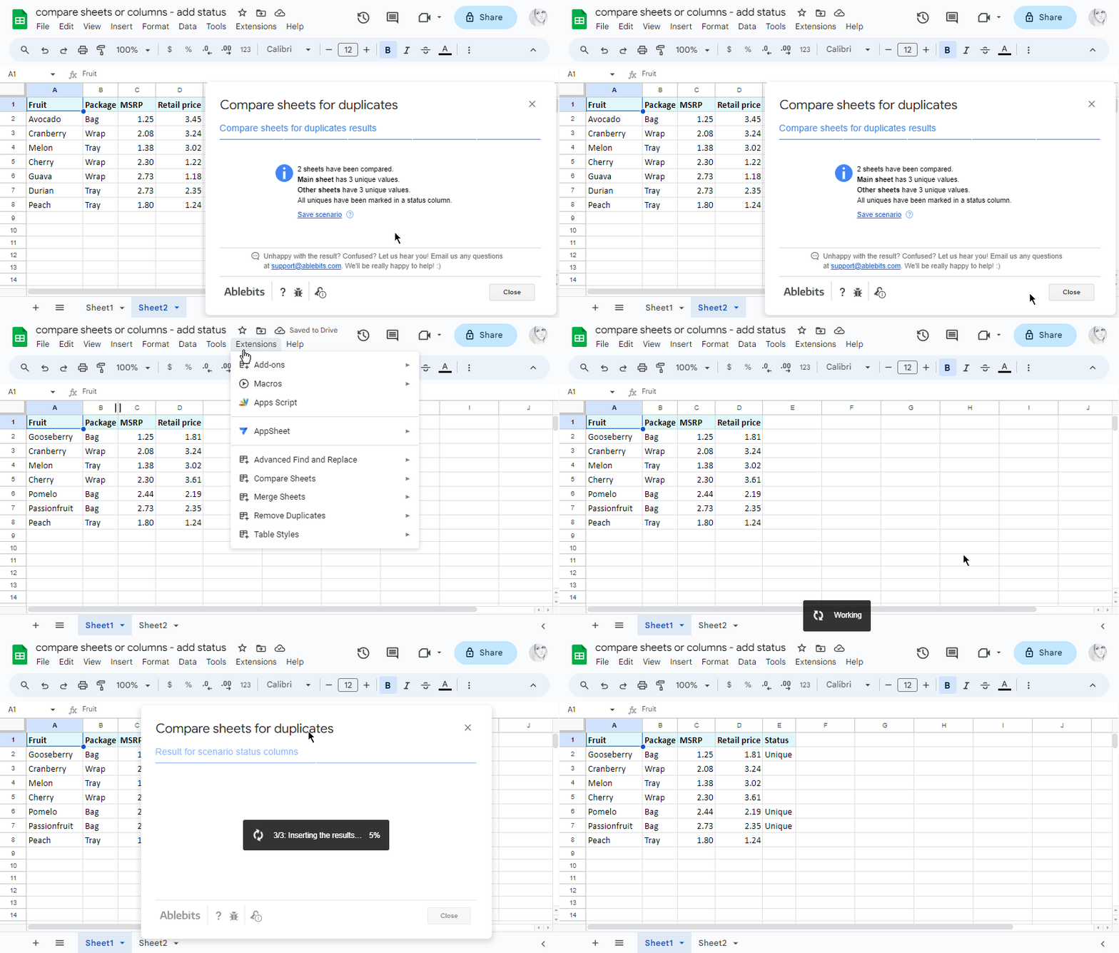
I used Compare Sheets to find the rows from Sheet1 that are absent from Sheet2 (and vice versa) based on Fruit and MSRP columns:

Then I saved my settings into one scenario. Now I can quickly run them without going through all steps again whenever records in my tables change. I just need to start that scenario from the Google Sheets menu:
This help page will gently guide you in case you're stuck on any step.
Compare sheets cell by cell
This on is also part of the Compare Sheets collection for Google Sheets.
It will compare your Google Sheets for differences. Whether you have two or more tables, it will check them all cell by cell and create one thorough report with differences from all sheets grouped accordingly.
Here's an example of the same two tables. The add-on creates one report with not only different cells (marked with yellow) but also unique rows (marked with red and blue):

Video: How to work with the comparison report
To look at the report and all its parts closely, feel free to read this tutorial or watch this demo video:
Compare data in two Google Sheets and fetch missing records
Comparing two Google Sheets for differences and repeats is half the work, but what about missing data? There are special functions for this as well, for example, VLOOKUP. Let's see what you can do.
Find missing data
Example 1
Imagine you have two lists of products (columns A and C in my case, but they can simply be on different sheets). You need to find those presented in the first list but not in the second one. This formula will do the trick:
=ISERROR(VLOOKUP(A2,$C:$C,1,0))
How does the formula work:
- VLOOKUP searches for the product from A2 in the second list. If it's there, the function returns the product name. Or else you will get an #N/A error meaning the value wasn't found in column C.
- ISERROR checks what VLOOKUP returns and shows you TRUE if it's the value and FALSE if it's the error.
Thus, cells with FALSE are what you're looking for. Copy the formula to other cells to check each product from the first list:

Note. If your columns are in different sheets, your formula will reference one of them:
=ISERROR(VLOOKUP(A2,Sheet2!$C:$C,1,0))
Tip. To get by with a one-cell formula, it should be an array one. Such formula will automatically fill all cells with results:
=ArrayFormula(ISERROR(VLOOKUP(A2:A10,$C:$C,1,0)))
Example 2
Another smart way would be to count all appearances of the product from A2 in column C:
=IF(COUNTIF($C:$C, $A2)=0, "Not found", "")
If there's absolutely nothing to count, the IF function will mark cells with Not found. Other cells will remain empty:

Example 3
Where there's VLOOKUP, there's MATCH. You know that, right? ;) Here's the formula to match products rather than count:
=IF(ISERROR(MATCH($A2,$C:$C,0)),"Not found","")
Tip. Feel free to specify the exact range of the second column if it remains the same:
=IF(ISERROR(MATCH($A2,$C2:$C28,0)),"Not found","")
Pull matching data
Example 1
Your task may be a bit fancier: you may need to pull all missing information for the records common for both tables, for example, update prices. If so, you'll need to wrap MATCH in INDEX:
=INDEX($E:$E,MATCH($A2,$D:$D,0))
The formula compares fruits in column A with fruits in column D. For everything found, it pulls the prices from column E to column B.

Example 2
As you may have guessed, another example would use the Google Sheets VLOOKUP function that we described some time ago.
Yet, there are a few more instruments for the job. We described them all in our blog as well:
Merge sheets using the add-on
If you're tired of formulas, you can use our Merge Sheets add-on to quickly match and merge two Google sheets.
Alongside its basic purpose to pull the missing data, it can also update existing values and even add non-matching rows. You can see all changes in colour or in a status column that can be filtered.
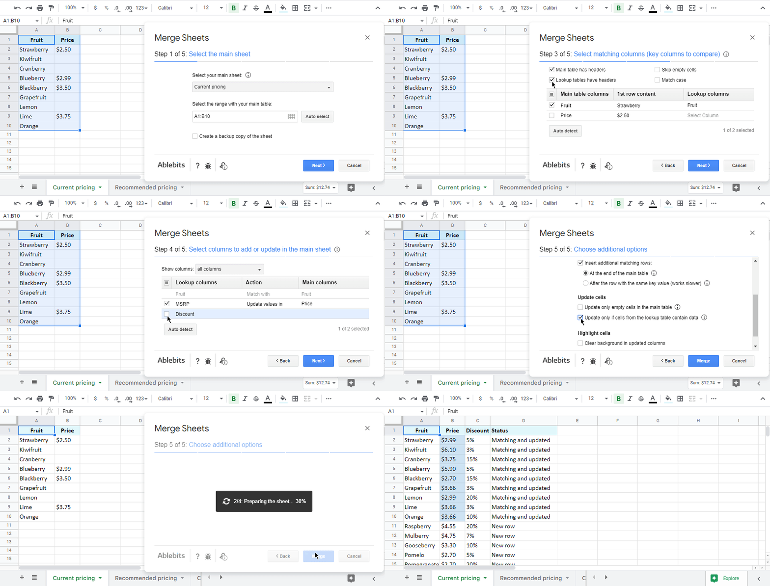
The 2.0 version of Merge Sheets will merge not just 2 tables (one main with one lookup) but multiple sheets in a row (one main with several lookups). The data from the lookup sheets will be added to your main one by one: as you added them in the add-on. Lots of additional options will make your merge as comprehensive as you need.
Video: How to use Merge Sheets add-on for Google Sheets
Check out this video about the Merge Sheets add-on. Though it features just 2 sheets, it paints a clear picture of the add-on possibilities:
Conditional formatting to compare data in two Google Sheets
There's one more standard way Google offers to compare your data – by colouring matches and/or differences via conditional formatting. This method makes all records you're looking for stand out instantly. Your job here is to create a rule with a formula and apply it to the correct data range.
Highlight duplicates in two sheets or columns
Let's compare two columns in Google Sheets for matches and colour only those cells in column A that tally with cells in the same row in column C:
- Select the range with records to color (A2:A10 for me).
- Go to Format > Conditional formatting in the spreadsheet menu.
- Enter a simple formula to the rule:
=A2=C2 - Pick the color to highlight cells.
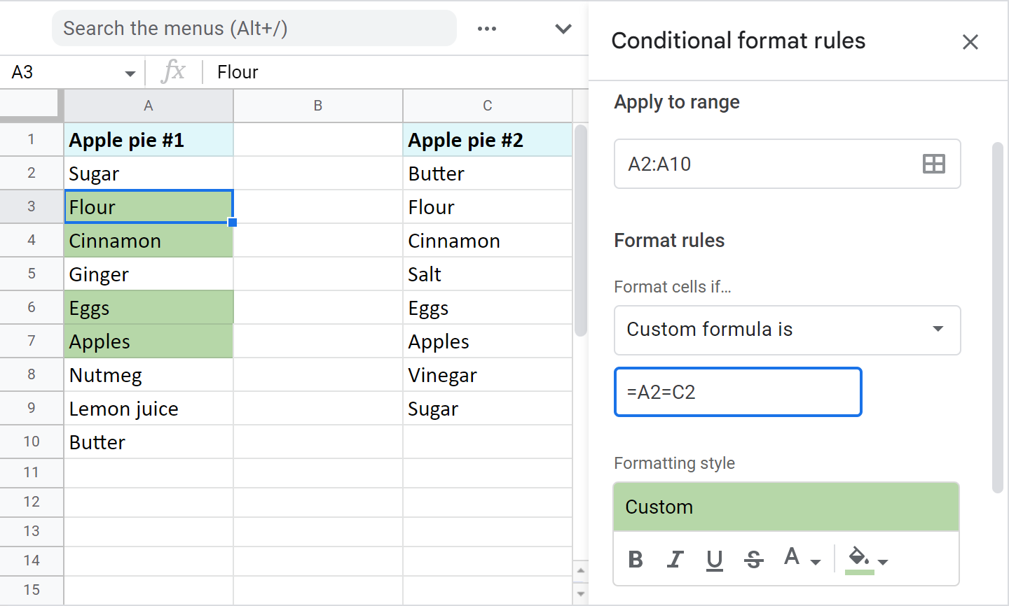
Tip. If your columns change in size constantly and you want the rule to consider all new entries, apply it to the entire column (A2:A, assuming the data to compare starts from A2) and modify the formula like this:
=AND(A2=C2,ISBLANK(A2)=FALSE)
This will process entire columns and ignore empty cells.
Note. To compare data from two different sheets, you'll have to make other adjustments to the formula. You see, conditional formatting in Google Sheets doesn't support cross-sheet references. However, you can access other sheets indirectly:
=A2=INDIRECT("Sheet2!C2:C")
In this case, please specify the range to apply the rule to – A2:A10.
Compare two Google sheets and columns for differences
To highlight records that don't match cells on the same row in another column, the drill is the same as above. You select the range and create a conditional formatting rule. However, the formula here differs:
=A2<>C2
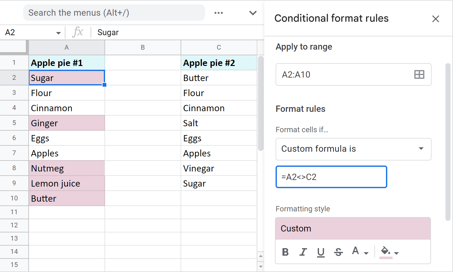
Again, modify the formula to make the rule dynamic (have it consider all newly added values in these columns):
=AND(A2=C2,ISBLANK(A2)=FALSE)
And use the indirect reference to another sheet if the column to compare with is there:
=A2<>INDIRECT("Sheet1!C2:C")
Note. Don't forget to specify the range to apply the rule to – A2:A10.
Compare two lists and highlight records in both of them
Of course, it's more likely the same records in your columns will be scattered. The value in A2 in one column will not necessarily be on the second row of another column. In fact, it may appear much later. Clearly, this requires another method of searching for the items.
Example 1. Compare two columns in Google Sheets and highlight differences (uniques)
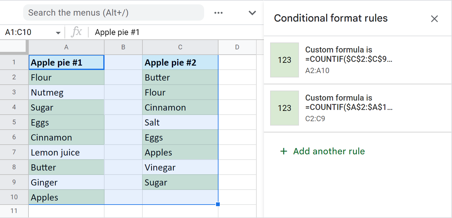
To highlight unique values in each list, you must create two conditional formatting rules for each column.
Color column A: =COUNTIF($C$2:$C$9,$A2)=0
Color column C: =COUNTIF($A$2:$A$10,$C2)=0
Here are the uniques I've got:

Example 2. Find and highlight duplicates in two columns in Google Sheets
You can colour common values after slight modifications in both formulas from the previous example. Just make the formula count everything greater than zero.
Color dupes between columns in A only: =COUNTIF($C$2:$C$9,$A2)>0
Color dupes between columns in C only: =COUNTIF($A$2:$A$10,$C2)>0
Tip. Find many more formula examples to highlight duplicates in Google Sheets in this tutorial.
3 quickest ways to match columns and highlight records
Conditional formatting can be tricky sometimes: you may accidentally create a few rules over the same range or apply colors manually over cells with rules. Also, you have to keep an eye on all ranges: the ones you highlight via rules and those you use in the rules themselves. All of these may confuse you a lot if you're not prepared and not sure where to look for the problem.
Luckily, our Compare Sheets collection for Google Sheets has 3 user-friendly solutions for you.
Video: What is Compare Sheets collection
Add-on to compare & highlight duplicates or uniques
Compare sheets for duplicates is intuitive enough to help you match different tables within one file or two separate files, and highlight those uniques or dupes that may sneak into your data.
Here's how I highlighted duplicates between just two tables based on Fruit and MSRP columns using the tool:
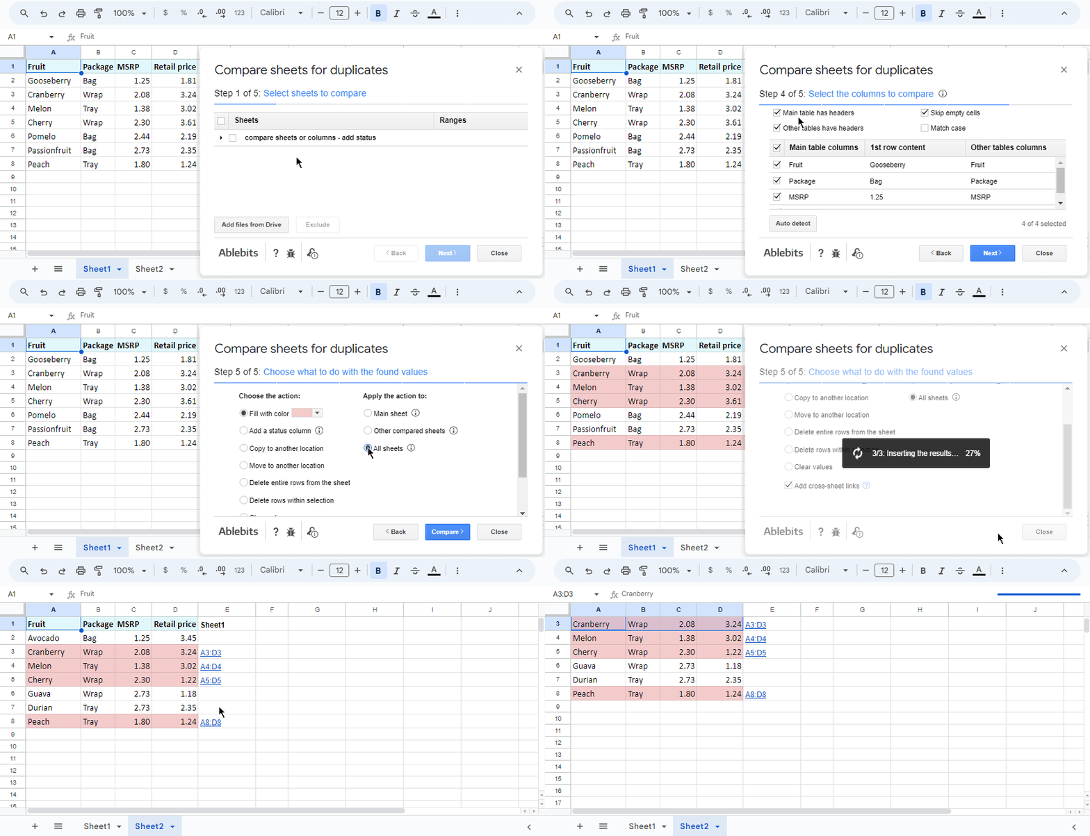
I can also save these settings into a reusable scenario. If the records update, I will call for this scenario in just a click and the add-on will immediately start processing all the data. Thus, I avoid tweaking all those settings over the add-on steps repeatedly. You will see how scenarios work in the example above and in this tutorial.
Add-on to compare Google sheets and highlight differences
Compare sheets cell by cell doesn't fall behind. It sees all differences between two columns or sheets. In fact, it compares as many sheets as you need, even from different files. Usually, one of these tables acts as your main one, and you compare it with others. The add-on highlights differences on those other sheets so you could spot them instantly:

Video: How to use Compare Sheets Cell by Cell add-on
This help page and the demo video below will give you a better idea of how it compares multiple Google sheets for differences:
Compare two columns and color dupes/uniques
This last tool comes in especially helpful for a simpler task: comparing just two columns within one Google tab. Why especially helpful? Because since both columns are on one sheet, going over 5 steps is too much. Hence, there's only one step with all the necessary settings:

This tutorial discusses every option in detail if you'd like to take a look.
And guess what? Compare Columns is also part of the Compare Sheets collection for Google Sheets.
That's right: you get all 3 tools with just one add-on. Give it a go and you won't regret it! (And if you do, let me know why in the comments section!)
Anyways, all these methods are now at your disposal – experiment with them, modify and apply them to your data. If none of the suggestions help your particular task, feel free to discuss your case in the comments down below.
 by
by
212 comments
I just want to highlight any value in one column that is great than the value in the column next to it. Can you please help?
Hello Wes,
Please read this tutorial on conditional formatting based on another cell to learn how to do that.
Hi!
I have data from 3 different databases, now in one spreadsheet, one database in each column A, B, C(C is the largets), and I need to erase from column C, all of the cells repited from columns A and B.
Could you help me?
Hi Mila,
Formulas won't erase the values. For that, consider using our Compare Two Columns tool and compare column C with column A then with column B.
HI,
I have two sheets that I am trying to match first and last names. Sometimes the first name (and rarely, the last name), may be misspelled but want them match. For example master sheet has Andy Jones, but other sheet says Andrew Jones, which is the same person
I have the following formula that only works when first and last names are perfectly matched.. But I want to capture slight variations
=IF(COUNTIFS(SheetA!$B:$B,A1,SheetA!$C:$C,BA1),"Yes","No")
I have tried to add the "*A1*" wildcards, but I get errors. Any help is appreciated!
Hi! To use wildcards in the COUNTIF and COUNTIFS functions, add "*" using the & operator. For example, "*"&A1&"*"
Thanks for this. How much variation does the wildcard give you? For instance if I have Richard Jones on the main sheet and I have Rich Jones on the second sheet, the wildcards do not flag that. Any suggestions?
Hi! I recommend paying attention to the Find Fuzzy Matches for Google Sheets tool. The tool compares words for similarities and differences and creates a list for you of all fuzzy duplicates grouped by entry.
looking to match a column of customer number with second sheet or added columns to the first sheet containing customer numbers and names- so I can see who needs to be contacted.
Hi! If I understand your task correctly, try to use VLOOKUP formula. Read more: VLOOKUP in Google Sheets with formula examples.
I am trying to identify changes in sheets I receive each month. Important data is customer id #, names, and a Yes/No column, plus there are a few columns I am not concerned about. I want to see when someone is no longer listed on the newer sheet (this is the one I am having the most trouble with), when there is a new person addition, and when someone has changed from yes to no. I'm unable to come up with a concise way to do all 3. Any advice would be greatly appreciated.
Hi! To compare Excel spreadsheets for differences, I'd recommend you to take a look at our Compare Sheets tool. It is available as a part of our Ultimate Suite for Excel that you can install in a trial mode and check how it works for free.
I have 2 spreadsheets with part numbers in column A. Each sheet is for a different company. Column B has the specific pricing for that company. Is there a way to combine these sheets so that I can see a column with the pricing for the first company and a column right next to it for 2nd company for each part number?
Hello Crystal,
There are a few ways, I described them in this part of the article, please take a look.
hi i have 2 columns filled with numbers. Lets call them Column A and Column B.
Column A represents my target and column B my current position, i would like to apply a colour scheme of red to column B if the numbers don't match the target and green if it does.
A B
1 0 (make red)
3 3 (make green)
7 6 (make red)
thank you
Hi Justin,
This solution will help you.
Hi, first of all thanks for your amazing work. I hope you can help me.
How can I reconcile 2 Excel sheets to make sure the data matches up? For example, two months of payroll. How can I have Excel compare both sheets and highlight where they differ (name/amount)?
How do I set it up so I know what the issue is? Ex. Red for extra names, yellow for contradicting numbers...
Thank you!
Hi Izzy,
Thank you for your feedback! For comparing files in Excel, please visit this article.
thank you so much
Hi,
I have a sheet with columns:
A - list of names in no particular order
B - list of names in no particular order
I want in a third column:
C - list of names that are in both column A and B (matching names, but since they won't necessarily be on matching rows, it needs to check for matches in the whole columns and just add in column C the names that do appear anywhere in both columns A and B).
Is there a formula for this that I could simply put in column C?
Or how would I go about producing a list in a separate column with only the matching names from A and B?
Thanks so much for any help!
Hi JN,
Try this formula:
=UNIQUE(FILTER(A:A, COUNTIF(B:B, A:A)))
Learn more about COUNTIF, FILTER & UNIQUE
What if I want the values that don't match in column C?
Try this one then:
=FILTER(A:A, ISNA(MATCH(A:A, B:B, 0)),A:A<>"")
Hello,
I have browsed through multiple of your tutorials and streamlined many of my worksheets using the techniques you have published. There is still some issues where I need assistance.
I own a business where we deliver goods to 150 consumers a day and have to track their online payments. Each consumer has a unique consumer id and the buying process involves the consumer booking and paying for the goods online and the goods are delivered to them in the next 1-2 weeks. Now we have a team of delivery personnel who deliver the goods to the consumers and bring back the consumer ids who have completed the payment. We verify the payments by extracting the consumer data from our company's online portal which contains the transaction details of all the consumers in the form of an elaborate list. We call it the portal list. We do the cross verifying on a monthly basis to avoid any discrepancy in payments from the Delivery team and the actual amount of the goods sold. The entries for the month are 4000+.
1. So now to verify we create two lists. One with all the consumer numbers obtained from the delivery boys (Lets call this list 'DList' ) and the second is the list of consumer ids we get from the portal (Lets call this 'PList' ). I use the following formula to compare the consumer id provided by the DBoy and compare it with the column in the Portal list which contains the Consumer ids we got from the portal.
=IF(ISNA(VLOOKUP(D2, PList!$E$2:$E$5000, 1, FALSE))," NOT RECIEVED", "RECIEVED")
I paste this formula in the DList in which the D column holds the consumer numbers provided by the DBoy. Then I get the list of consumers who's payment has been received and who's is not (The discrepancy over here is that the DBoys might provide a fake number or a wrong one and there is a possibility of theft.)
But this formula fails if the consumer has taken the goods more than once in a month because the formula only compares and returns the value of 'RECIEVED' even if the consumer id matches the PList just once. So to count the number of matches I use the following formula.
=SUMPRODUCT(COUNTIF(D2,PList!$E$2:$E$5000))
This shows me if the consumer id provided by the Dboy has 1 matches or >1 and then we can verify the consumers who have got the goods more than once in a month by finding the consumer id in the PList manually (Using Ctrl + F and then pasting the respective consumer id in the Find Popup) and verifying if the consumer id provided by the DBoy is legit.
But this process takes a lot of time and effort for us to complete.
So I wanted a formula which compares the Consumer id in the Dlist with the Column of Consumer id in the PList and then returns with the values which match and the values which don't match. I also need the formula to highlight the Row in Plist which shows more than one matches with the Consumer IDs in the DList and if possible create a separate table with those highlighted rows in a different table in the same worksheet.
Hello,
I'm glad to hear our articles help you with your spreadsheets!
Now, thanks to your thorough and detailed description I understand the whole workflow and the formulas you're using. What I'm having difficulties to get is the exact result you'd like to see. I'm not sure but it looks like you're trying to compare the IDs row by row on these sheets, as described in this part of the article?
If not, please create a sample sheet with about 20 rows of user IDs samples in each list (don't have to be the real ones) & with the example of the result you'd like to get from these lists. And share this sample with us: support@apps4gs.com. I'll look into it and try to help.
Note. We keep that Google account for file sharing only and don't monitor its Inbox. Please do not email there. Once you share the file, just confirm by replying to this comment.
As for highlighting, I believe the COUNTIF formulas like here in the Example 2 will help you out. You just need to use the '>1' condition instead of '>0'
Date Open
Feb-02-2007 273.85
Feb-05-2007 324.65
Feb-06-2007 307.1
Feb-07-2007 347.86
Feb-08-2007 381.42
Feb-09-2007 355.36
Feb-12-2007 346.59
Feb-13-2007 302.72
Feb-14-2007 302.72
Feb-15-2007 319.08
Feb-19-2007 368.35
Feb-20-2007 356.85
Feb-21-2007 347.9
I want to fill missing dates with zero value example, how to do it, please guide me.
Date Open
Feb-02-2007 273.85
Feb-03-2007 0
Feb-04-2007 0
Feb-05-2007 324.65
Feb-06-2007 307.1
Thanks, Rishi
Hello Rishi,
I'm afraid there's not formula that would add rows inside your table and fill them with the required dates and values. You may try to find a solution here – an overview of Google Apps Script with a lot of helpful content and links:
https://developers.google.com/apps-script/overview
Is it possible to highlight duplicates over several tabs in excel and google sheets?
I have a tab/sheet per day and I need a range of 3 columns to indicate if there are any duplicate entries.
Hello Tina,
If you work in Google Sheets, the first two ways that describe highlighting duplicates are fit for comparing more than 2 sheets at a time. The third way with conditional formatting will require several rules where you compare 2 sheets a time. We are also working on the add-on that will compare multiple tables at once.
Hello,
Thank you for your blog!
I'm looking for the formula for INDEX MATCH MATCH in Google sheets.
The 'Pull matching data' but with two criteria
Hello Louis,
If I understand you correctly, you're looking for this solution.
Hi!
I hope you are able to help me.
I need to compare 2 columns if both have values or only 1 column has, how do I do it? Thanks in advance! You are really helping a lot of us! :)
Hi April,
Could you please describe the task in more detail? How do you want to see the results? Also, did you try any of the ways described in this article?
Hi I have three sheets of attendees for an event over the years (2020, 2021, and 2022). I want to find anyone who has attended ALL THREE years, so there would be a common value on each sheet. Email is the easiest value to compare. I can't find an applicable formula. I'd like to keep the data in Google sheets since another person needs access to it. Any suggestions?
Hi Tery,
Are the names in different tabs within the same file or in different files? Would you like to color the matching names in each sheet or pulled to other table?
Hi natialia hope that you can help me with the same about emails i just need to highlight the people attending to an event from a registration link to list of participants,
Hi andrea,
Have you tried methods described in this part of the article?
Hey there,
I have an accounting workbook with a sheet for Expenses, with a column for Descriptions with details of the charges (i.e. "Payment to Amazon", etc...).
I also have a Provider sheet that has my providers' names, details, etc... and includes a "Query" column with possible values to match against the Descriptions column in the Expenses sheet (i.e. "Amazon").
I want to automatically compare the values from the Expenses/Descriptions column with the Providers/Query column and if there is a match return the index of the row from Providers so that I can populate other fields in the Expense line with a VLOOKUP. The Query values might not be exact. They just have to match part of the string.
I've searched around a bit and I can find pieces of the puzzle but I'm not sure the best way to put it all together.
Is this possible? Any advice is greatly appreciated!
Hey Craig,
To look for partial matches, you need to use wildcard characters. Svetlana described them in this blog post, please have a look.
How do you compare 2 columns on 2 different tabs in the same Google Sheet for differences?
Hello George,
Feel free to use any of the ways described above: using formulas and a status column, using the add-on, or using colors.
Hi, Ablebits!!! Your wotk arr awesome. I was looking gor specific work to be carried using query formula. And my search was fullfiled after reading this page.. Thanks a lot.. Now i have learnet too further how to reduce the pain while handling multiple wotksheets.. Thank you team.. All the best, May God bless you
Hi Jaisankar,
Appreciate your feedback! Glad the article has helped! :)
Is it possible to distribute a column based on the text in another column?
Column has A:
50 blue
70 orange
100 red
Column B is longer:
50 tom
60 mike
70 betty
90 jace
100 natalia
110 glen
Desired Column c:
50 blue 50 tom
60 mike
70 orange 70 betty
90 jace
100 red 100 natalia
110 glen
I'm trying to distribute the info in column A to line up with Column B based on the unique of the number they both have... It's hard to explain.
Hello Eric,
I'd solve this task the following way:
Hi,
I'm curious if you could help me with the issue I'm running across. We provide services to young adults and have a list of the the services we've provided to each young adult (some young adults have had 10+ services this program year so they have 10+ rows in our sheet). We're being asked to provide the number of unique young adults served per quarter who did not receive services in the previous quarters of that same program year.
Our list includes names and dates of services. I can't figure out how to get the counts we need from our complete list so I split the names into 3 columns, each column containing the list of participants served each quarter (e.g. column 1 has Q1 participants, column 2 has Q2 participants, etc.) I then used the conditional formatting formula to highlight the participants served in Q2 who were not served in Q1 so that I could count them manually. The issue I'm running into is then figuring out the number of participants served in Q3 who were not served in Q1 and Q2. Our staff has always done this manually and I'm hoping we can use formulas to get these counts instead.
Here is a link to a sample spreadsheet: https://docs.google.com/spreadsheets/d/1qTLtGoPdfymhGZkHzuKy97VLwXXPpZTBJapsFV1IXcY/edit?usp=sharing
Hi Natalie,
Thank you for sharing the file right away.
I duplicated the Students by quarter sheet and put the results there, please take a look.
Natalia. Thank you so much for this. Those formulas to pull over the de-duplicated data are incredibly helpful. With that and the conditional formatting rules, we'll be able to get those final numbers much quicker.
Thank you so much for your help!
I'm happy to help, Natalie! :)