The IF function in Google Sheets is one of the easiest functions to learn, and while this holds true, it is also a very helpful one.
In this tutorial, I invite you to take a closer look at how Google Spreadsheet IF function works and what advantages you will get from using it.
What is the IF function in Google Sheets?
Whenever you use the IF function, you create a decision tree in which certain action follows under one condition, and if that condition is not met – another action follows.
For this purpose, the condition of the function must be in a format of the alternative question with only two possible answers: "yes" and "no".
This is what a decision tree may look like:
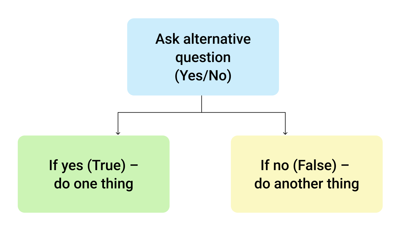
So, the IF function allows you to ask a question and indicate two alternative actions depending on the received answer. This question and the alternative actions are known as three arguments of the function.
IF function syntax in Google Sheets
The syntax for the IF function and its arguments are as follows:
- logical_expression – (required) a value or logical expression that is tested to see if it is TRUE or FALSE.
- value_if_true – (required) the operation that is carried out if the test is TRUE.
- value_if_false – (optional) the operation that is carried out if the test is FALSE.
Let's explore the arguments of our IF function in more detail.
The first argument represents a logical question. Google Sheets answers this question with either "yes" or "no", i.e. "true" or "false".
How to formulate the question properly, you may wonder? To do that, you can write a logical expression using such helpful symbols (or comparison operators) as "=", ">", "<", ">=", "<=", "<>". Let us try and ask such a question together.
Usage of the IF function
Let's assume that you are working in the company selling chocolate in several consumer regions with many clients.
This is what your sales data may look like in Google Sheets:
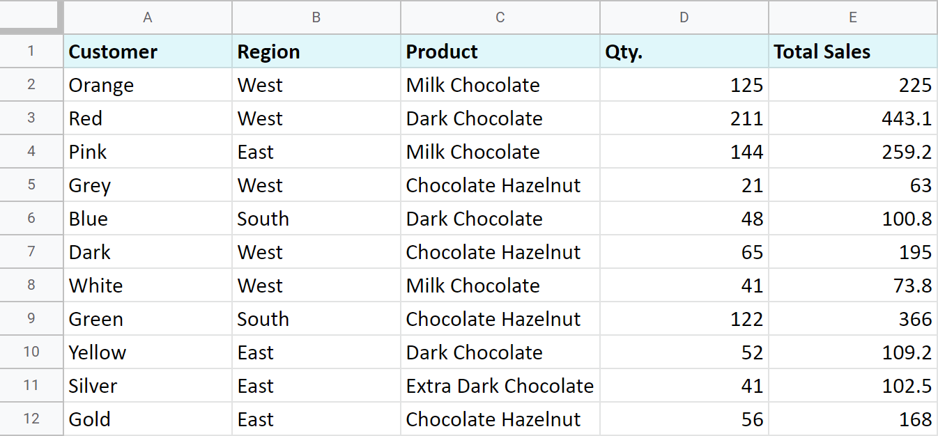
Imagine that you need to separate sales made in your local regions from those from abroad. To accomplish that, you should add another descriptive field for each sale – a country where the sales took place. Since there is a lot of data, you need this description field to be created automatically for each entry.
And this is when the IF function comes to play. Let's add the "Country" column to the data table. "West" region represents local sales (Our Country), while the rest are the sales from abroad (Rest of the World).
How to write out the function properly?
Place the cursor in F2 to make the cell active and type in the equality sign (=). Google Sheets will immediately understand that you are going to enter a formula. That's why right after you type the letter "i" it will prompt you to choose a function that begins with that same letter. And you should choose "IF".
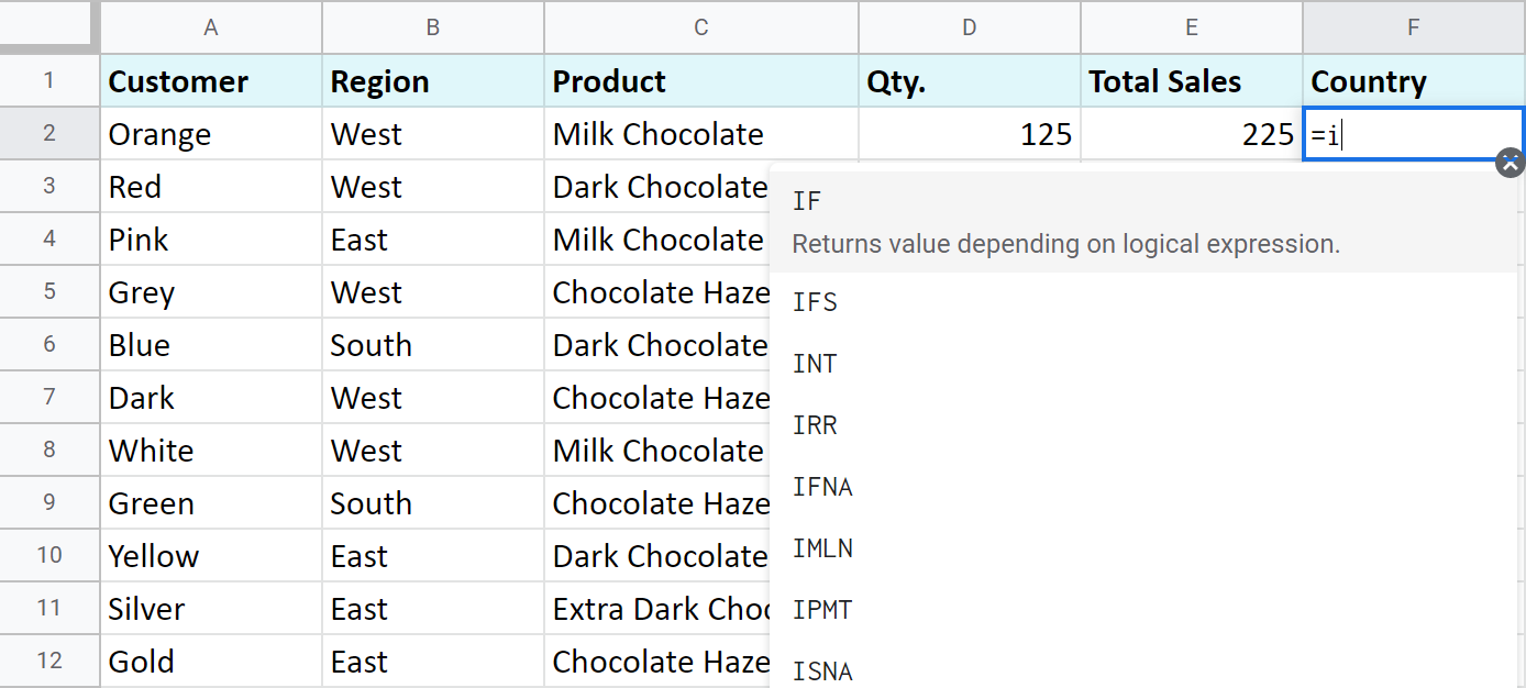
After that, all your actions will be accompanied by prompts as well.
For the first argument of the IF function, enter B2="West". As with the other Google Sheets functions, you don't need to enter the address of the cell manually – a mouse click is enough. Then enter comma (,) and specify the second argument.
The second argument is a value that F2 will return if the condition is met. In this case, it will be the text "Our Country".
And again, after the comma, write the value of the 3rd argument. F2 will return this value if the condition is not met: "Rest of the World". Do not forget to finish your formula entry by closing parenthesis ")" and pressing "Enter".
Your entire formula should look like this:
=IF(B2="West","Our Country","Rest of the World")
If everything is correct, F2 will return the text "Our Country":
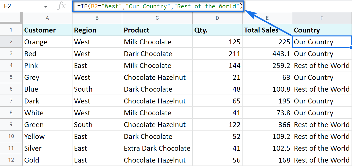
Now, all you have to do is to copy this function down column F.
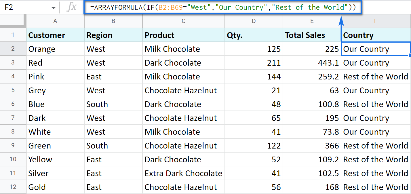
Tip. There's one way to process the entire column with one formula. The ARRAYFORMULA function will help you do that. Using it in the first cell of the column, you can test all cells below against the same condition, and return the corresponding result to each row at the same time:
=ARRAYFORMULA(IF(B2:B69="West","Our Country","Rest of the World"))
Let's examine the other ways of working with the IF function.
IF function and text values
The usage of the IF function with a text has already been illustrated in the example above.
Note. If the text is being used as the argument, then it must be enclosed in double-quotes.
IF function and numerical values
You can use numbers for the arguments just as you did with the text.
However, what is very important here is that the IF function makes it possible to not only fill cells with certain numbers based on the conditions met but also calculate.
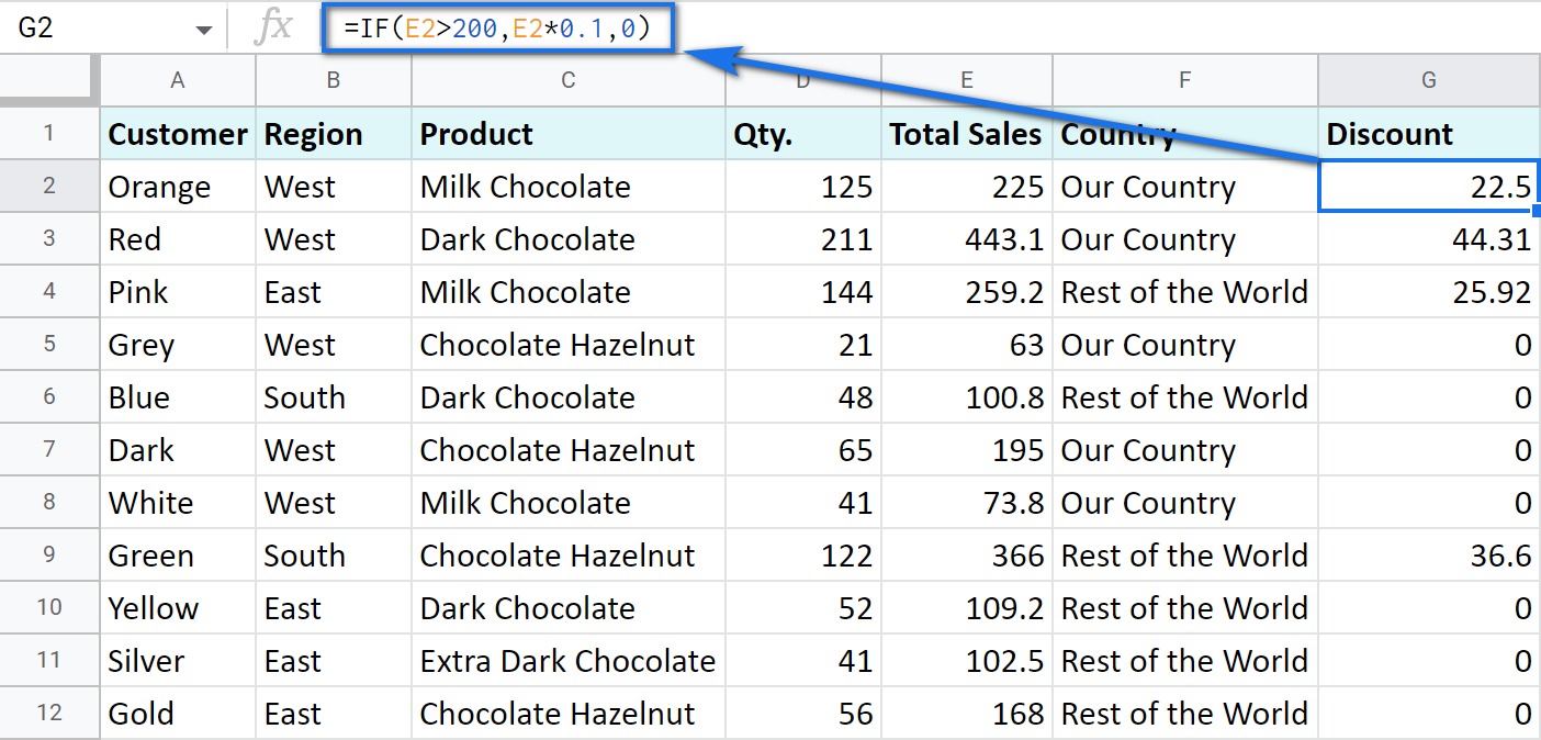
For example, let's say you offer your clients various discounts based on the total value of the purchase. If the total is more than 200, then the client gets a 10% discount.
For that, you need to use column G and name it "Discount". Then enter the IF function in G2, and the second argument will be represented by the formula that calculates the discount:
=IF(E2>200,E2*0.1,0)
IF blanks/non-blanks
There are cases when your result depends on whether the cell is empty or not. There are two ways to check that:
- Use the ISBLANK function.
For example, the following formula checks if cells in column E are empty. If so, no discount should be applied, otherwise, it's 5% off:
=IF(ISBLANK(E2)=TRUE,0,0.05)
Note. If there's a zero-length string in a cell (returned by some formula), the ISBLANK function will result in FALSE.
Here is another formula to check if E2 is empty:
=IF(ISBLANK(E2)2<>FALSE,0,0.05)You can turn the formula the other way around and see if cells are not blank instead:
=IF(ISBLANK(E2)=FALSE,0.05,0=IF(ISBLANK(E2)<>TRUE,0.05,0) - Use standard comparison operators with a pair of double-quotes:
Note. This method considers zero-length strings (indicated by double-quotes) as empty cells.
=IF(E2="",0,0.05)– check if E2 is blank=IF(E2<>"",0,0.05)– check if E2 is not empty.Tip. In a similar manner, use double-quotes as an argument to return an empty cell by the formula:
=IF(E2>200,E2*0,"")
IF in combination with other functions
As you have already learned, the text, numbers, and formulas can act as the arguments of the IF function. However, other functions can play that role as well. Let's see how it works.
Google Sheets IF OR
Remember the first way you figured out the country where you sold chocolate? You checked if B2 contained "West".
However, you can build the logic the other way around: list all the possible regions that belong to the "Rest of the World" and check if at least one of them appears in the cell. The OR function in the first argument will help you do that:
- logical_expression1 – (required) the first logical value to check for.
- logical_expression2 – (optional) the next logical value to check for.
- and so on.
As you can see, you just enter as many logical expressions as you need to check and the function searches if one of them is true.
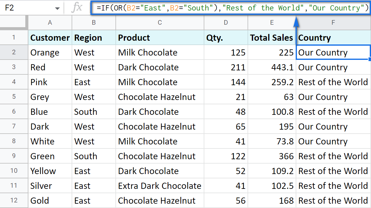
To apply this knowledge to the table with sales, mention all the regions that belong to the sales abroad, and the other sales will automatically become local:
=IF(OR(B2="East",B2="South"),"Rest of the World","Our Country")
Google Sheets IF AND
The AND function is just as simple. The only difference is that it checks if all listed logical expressions are true:
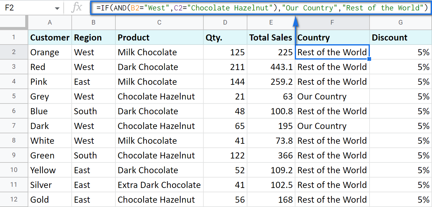
E.g. you need to narrow the search to your town and you know that it is currently buying only hazelnuts. So there are two conditions to consider: region – "West" and product – "Chocolate Hazelnut":
=IF(AND(B2="West",C2="Chocolate Hazelnut"),"Our Country","Rest of the World")
Nested IF formula vs. IFS function for Google Sheets
You can also use the IF function itself as an argument for the bigger IF function.
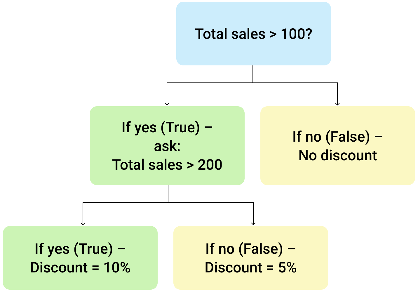
Let's assume that you have set stricter discount conditions for your clients. If the total purchase is more than 200 units, they get a 10% discount; if the total purchase is between 100 and 199, the discount is 5%. If the total purchase is lower than 100, there is no discount whatsoever.
The following formula shows how the function will look in the cell G2:
=IF(E2>200,E2*0.1,IF(E2>100,E2*0.05,0))
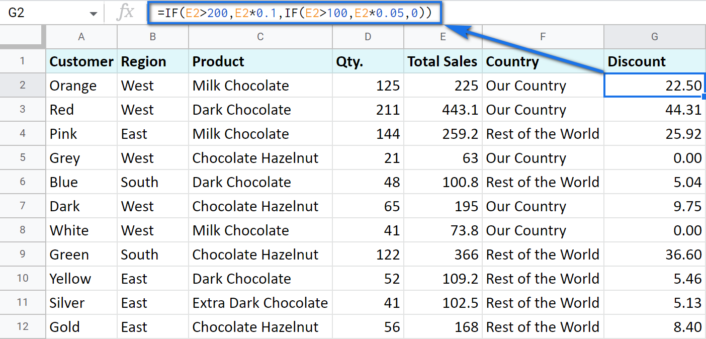
Note that it is another IF function that is used as the second argument. In such cases, the decision tree is as follows:
Let's make it even more fun and complicate the task. Imagine that you're offering the discounted price to the one region only - "East".
To do that correctly, add the logical expression "AND" to our function. The formula will then look the following way:
=IF(AND(B2="East",E2>200),E2*0.1,IF(AND(B2="East",E2>100),E2*0.05,0))
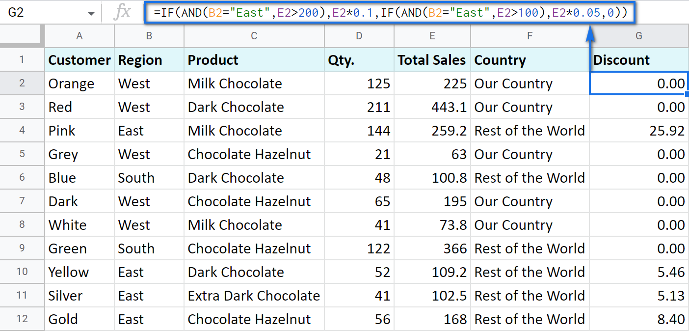
As you can see, the number of discounts has reduced greatly while their amount remains intact.
There's also an easier way to write the above thanks to the IFS function:
- condition1 – (required) is the logical expression you want to test.
- value1 – (required) is the value to return if the condition1 is true.
- and then you just list conditions with their values to return if they are true.
Here's how the above formula will look with IFS:
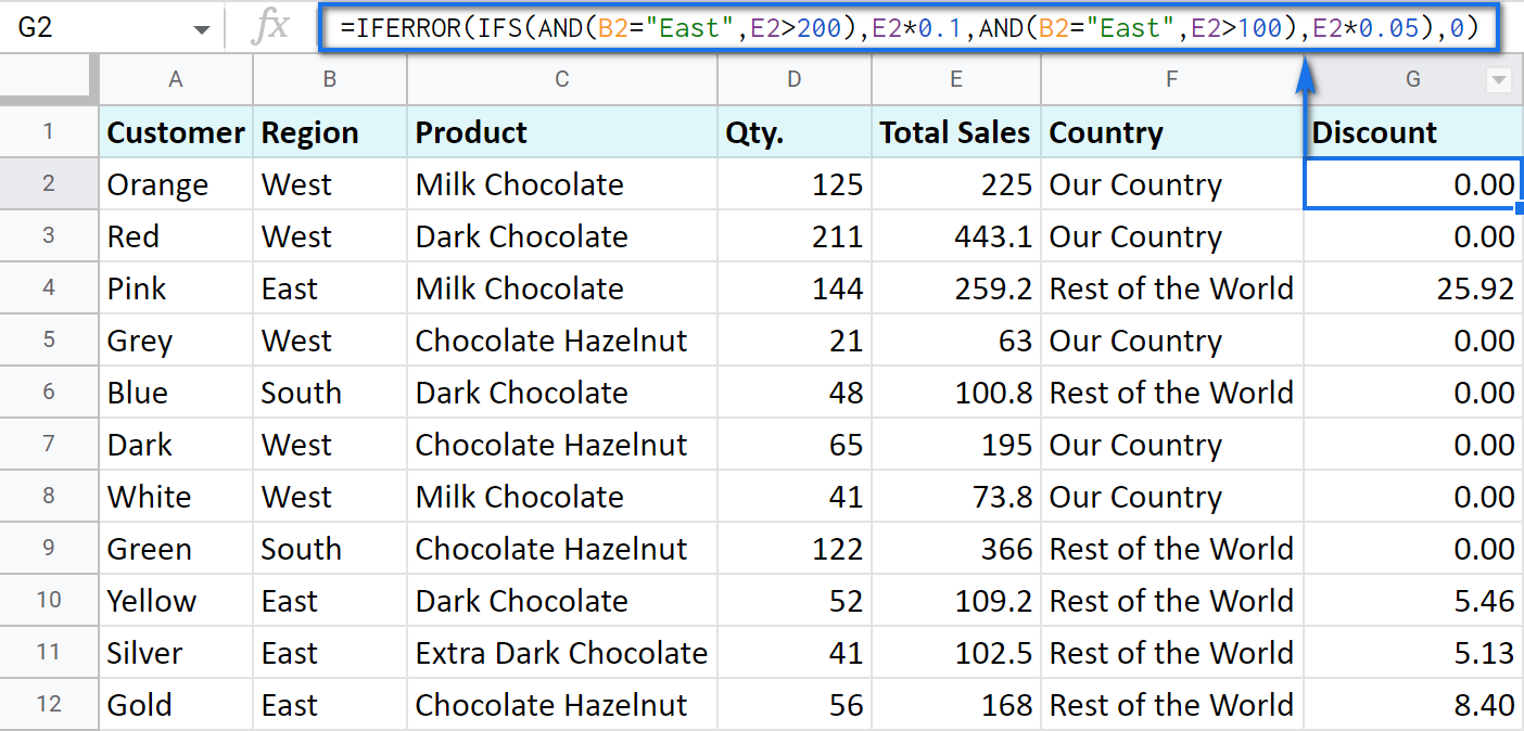
=IFS(AND(B2="East",E2>200),E2*0.1,AND(B2="East",E2>100),E2*0.05)
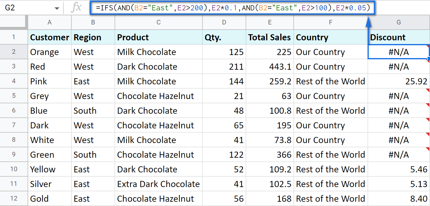
Tip. If there's no true condition, the formula will return the #N/A error. To avoid that, wrap your formula with IFERROR:
=IFERROR(IFS(AND(B2="East",E2>200),E2*0.1,AND(B2="East",E2>100),E2*0.05),0)
SWITCH as an alternative to multiple IFs
There's one more function you may want to consider instead of the nested IF: Google Sheets SWITCH.
It checks if your expression corresponds to a list of cases, one by one. When it does, the function returns a corresponding value.
- expression is any cell reference, or a range of cells, or even an actual math expression, or even a text that you'd like to equal to your cases (or test against the criteria). Required.
- case1 is your first criteria to check the expression against. Required.
- value1 is a record to return if the case1 criterion is the same as your expression. Required.
- case2, value2 repeat as many times as criteria you have to check and values to return. Optional.
- default is also completely optional. Use it to see a specific record if none of the cases is met. I'd recommend using it every time to avoid errors when your expression doesn't meet matches among all the cases.
Here are a couple of examples.
To test your cells against a text, use ranges as an expression:
=ARRAYFORMULA(SWITCH(B2:B69,"West","Our Country","Rest of the World"))
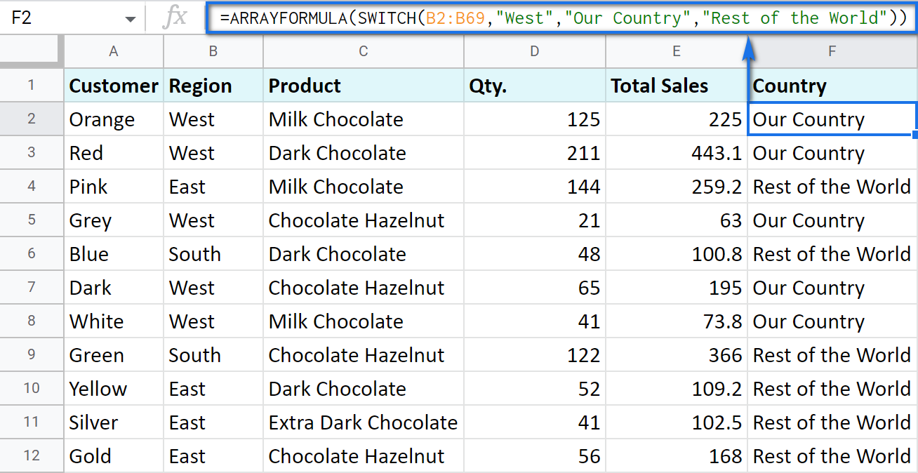
In this formula, SWITCH checks what record is in every cell in column B. If it's West, the formula says Our Country, otherwise, Rest of the World. ArrayFormula makes it possible to process the entire column at once.
To work with calculations, it's better to use a boolean expression:
=SWITCH(TRUE,$E2>200,$E2*0.1,AND($E2<200,$E2>100),$E2*0.05,0)
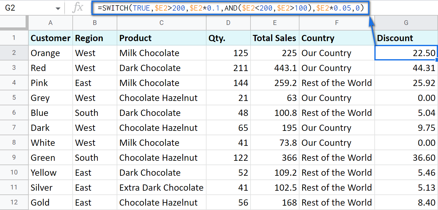
Here SWITCH checks if the result of the equation is TRUE or FALSE. When it's TRUE (like if E2 is really greater than 200), I get a corresponding result. If none of the cases in the list is TRUE (meaning they are FALSE), the formula simply returns 0.
Note. SWITCH doesn't know how to calculate the entire range at once, so no ARRAYFORMULA in this case.
IF statements based on a count
One of the questions we get asked a lot is how to create the IF formula that will return whatever you need if the column contains or doesn't contain a certain record.
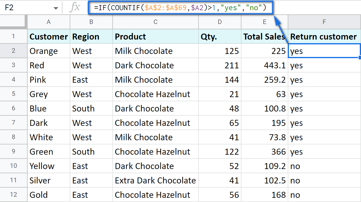
For example, check if a customer's name appears more than once in a list (column A) and put the corresponding word (yes/no) into a cell.
A solution is simpler than you may think. You need to introduce the COUNTIF function to your IF:
=IF(COUNTIF($A$2:$A$69,$A2)>1,"yes","no")
Make Google Sheets build IF formulas for you – IF Formula Builder add-on
If you're tired of keeping track of all those extra characters and proper syntax in formulas, there's another solution available.
IF Formula Builder add-on for Google Sheets offers a visual way of creating IF statements.
The tool will handle syntax, extra functions and all required characters for you.
All you need to do is:
- fill blanks with your records one by one. No special treatment for dates, time, etc. Enter them as you always do and the add-on will recognize the data type.
- select required comparison operators from the suggested drop-down lists.
- if needed, add multiple logical expressions in a click: IF OR, IF AND, ELSE IF, THEN IF.
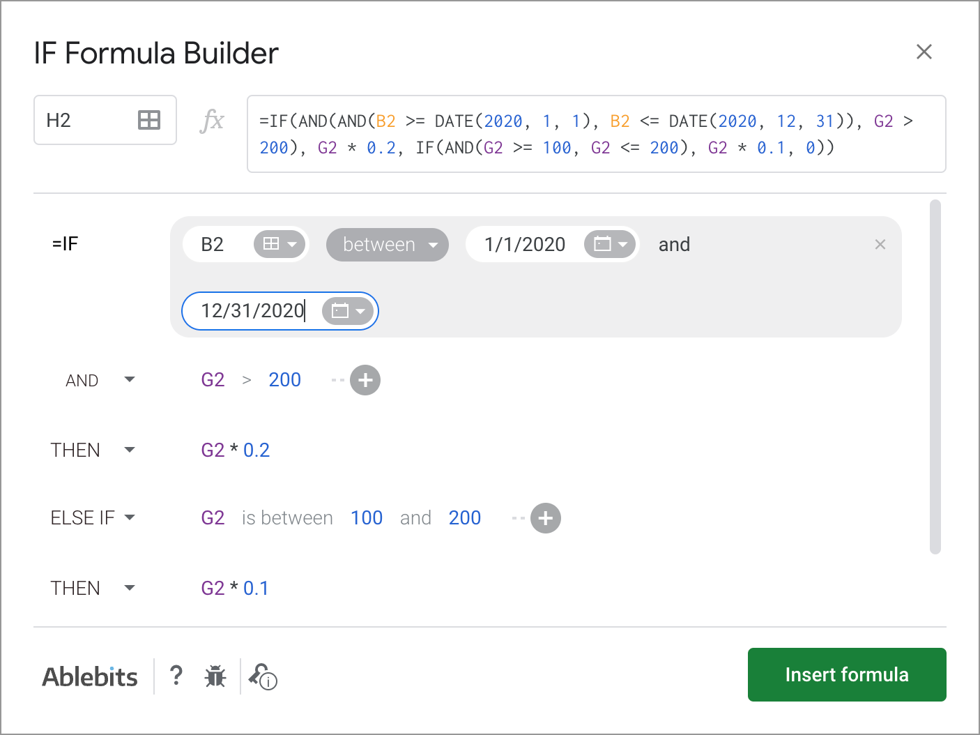
As you can see, each logical expression takes its own line. The same goes for true/false outcomes. This reduces the number of possible confusion over the formula drastically.
As you fill everything out, the formula for use will grow in the preview area at the top of the window. To its left, you can select a cell in your sheet where you'd like to have the formula.
When you're ready, paste the formula into the cell of interest by clicking the Insert formula button at the bottom.
Please visit the online tutorial for IF Formula Builder to see all options described in detail.
I hope that there's no room for any doubt now that the IF function, though a very simple one at first glance, opens the door to many options for data processing in Google Sheets. But if you still have questions, feel free to ask them in the comments section down below – we'll be happy to help!
 by
by
553 comments
I do not get it. What is wrong with this formula, the simplest of them all?... =IF(H27>=2,”Yes”,”No”). I get Error! ???
I have never tried to do formulas in a google sheet before, this is my first time, but I have done thousands in excel. I am confused. Is there anything I should know, anything I ,missed?
Humbly
Lena
Hello Lena,
Please specify what error you're getting exactly and what it says when you hover your mouse over it.
It says #ERROR
When hovering over this I get a swedish message
Fel
Fel i formeltolkning.
Which should render in direct translation
Error
Error in formula interpretation
It looks like you have a Swedish locale in this spreadsheet which requires semicolons (;) instead of commas (,) in formulas. Hence, the correct formula for you would be
=IF(H27>=2;"Yes";"No")
Alternatively, you can switch the locale to UK for example, to use formulas with the comma instead.
Aha! That explains the trouble. Now I know my options. Thanks a lot!
You're most welcome, Lena, glad I could help!
I am trying to write an if then formula for google sheets where if <40 then = 310040, if between 40 and 99 then = 310099, if between 100 and 249 then = 310249, if between 250 and 499 then = 310499, if 500 or greater then = 310500. This is what I have but its not working:
=IF(A1<40, 310040,
IF(A1<100, 310099,
IF(A1<250, 310249,
IF(A1<500, 310499,
310500))))
Can you help me?
Hello Craig,
Your formula doesn't work because you doesn't specify that numbers should be between other numbers AND(A1>40, A1<100), you're simply looking for everything less than smth and eventually each next argument is in conflict with all the previous ones. Here's the correct formula:
=IF(A1<40, 310040, IF(AND(A1>=40, A1<100), 310099, IF(AND(A1>=100, A1<250), 310249, IF(AND(A1>=250, A1<500), 310499, 310500))))
Please read this section of the article to learn how this works.
Hey there,
We have one product that offers three different pricing options.
Option1> SM Max
Option2> SM Ultra
Option3> SM Edge
all the prices include the GST amount, e.g. the Max plan cost is 11,800 INR (with 18% GST). Now, I want the result from this formula so that all the plan prices exclude the GST amount.
=IFS(AND(H148="Sm Max",I148="11,800"),"","10,000",AND(H148="SM Ultra",I148="23,600","","20,000",AND(H148="SM Edge",I148="47,200","","40,000)")))
When I apply this formula in my spreadsheet, it shows me an error message: "Function IFS parameter 3 expects boolean values. But '10,000' is a text and cannot be coerced to a boolean."
Let me know how to correct the formula.
Thank you
Yash
Hello Yash,
You're getting this error because of the incorrect syntax and the formula logic in general. As described here, the IFS function expects pairs of conditions and results. A second condition should be stated where you have "10,000".
If I understand your task correctly, the following corrected formula should do the trick:
=IFS(AND(H148="SM Max", I148="11,800"), "10,000", AND(H148="SM Ultra", I148="23,600"), "20,000", AND(H148="SM Edge", I148="47,200"), "40,000")
Yet, if numbers in double quotes should appear as numbers that you can calculate further, remove double quotes around them since double quotes are used to return text.
im trying to inout the if formular for if a cell is less than a certain value the the other cell is equal to the amount
i.e =if(P52<"85000", P52="85000") I keep getting a false
Hello Ruth,
Remove double quotes from numbers - they're used for text values only. Please see an example in this part of the article: IF function and numerical values
How do I highlight a certain if the value of another cell says a certain thing.
Hello Joel,
Please see this article: Create Google Sheets conditional formatting based on another cell
If you still need help, please describe your task in detail, I'll try to help.
Hi! I'm trying to do a complex IF using "NO" or "YES" to determine numbers.
Currently I have: =IF(AND($G$21="NO",$G$21="YES")," ", "1.5")
This only works for YES, not NO.
I've tried an IF(OR( but that didn't work. Any help would be greatly appreciated!
Hi Karissa,
I strongly believe it should be OR rather than AND because your G21 can show either NO or YES, not both at the same time in one cell if I understand the task correctly. Please provide the exact formula that doesn't work if you use OR - perhaps, something else is missing there. And specify what error it returns and what it says when you hover your mouse over the error.
I am trying to highlight a cell if another cell has particular word. Could you please help me with the code? Thank you so very much!
Hello Geetha,
You will find formula examples in this article: How to work with conditional formatting in Google Sheets
Im using the match() formula, how can i use the if() formula to get it to say "open" if the match() formula returns a value of N/A? (not the text N/A, its returning N/A because the match() formula cant find what its looking for by design.
Hello cody,
To replace errors with your own text, use the IFERROR function.
I'm sure its a simple function but I am learning. Thanks in advance for any help you can give.
The spreadsheet I am working on has a list of zip codes. A lot of them have duplicates. I want to create another row that will list the population density. I want to make a function that says if this zip code then this population density so as I add to the list if its a previously worked on zip code it will automatically add the population density.
Where my mind is currently at is I made a separate sheet, copied and pasted the zip codes in row A, deleted duplicates, looked up and entered population density in row B.
This is where I found a dead end and google suggests =IF formula but clearly I am doing something wrong.
Hello Tyler,
If I understand your task correctly, I think you need XLOOKUP function. It will match the codes you enter on one sheet with the codes written in a row in another sheet, and will pull the corresponding numbers from the rows below.
Hello,
I'm looking for a simple formula to show me the difference in values between 2 cells. I'd like it to indicate the negative differential if the value of cell B is lesser than cell A and remain 0 or empty if no values are entered in both cells.
Currently, I'm using =(E18)-(F18) but it's not indicating the - sign when the values return.
Kindly help.
Thanks
Hello Temi,
Please see how to compare numbers in the IF function in this part of the article.
If you still have any questions, please provide examples of your numbers and the desired output, I'll try to help.
Hello, In your first example under the "IF function and numerical values" section. If you wanted cell G2 "Discount", to display "Discount is 22.5". How would you modify the formula =IF(E2>200,E2*0.1,0)? I haven't been able to find how to combine text and a mathematical operation together. I would appreciate your help very much. Thank you in advance.
Hello Laura,
The CONCATENATE function will help you with that:
=IF(E2>200,CONCATENATE("Discount is "&E2*0.1,0)
Trying to make a if statement read a total based on individual cells. Example if a1>=6, +1 to d1, if b1>= 4, +1 to d1, if c1>=3, +1 to d1; total is in d1.
Also with above setting d1=0 to start the loop
Hello Jamaal,
Please look through this part of the article to build the formula that will solve your task.
=IF(C4>=18,I4+1, IF(E4>=5,I4+1,IF(G4>=2,I4+1,I4+0)))
Here is the code I have. The problem I am running into is that my total does not reset. For example: if I put in data the code runs and get a total of 2 per say. Then if I change an entry that should give me a total of 1 I get 3. It adds to what is in my total column instead of resetting to 0 first. Also if I start another row the previous row runs another loop and adds to that total again and the new row. Would love to share my doc with you if that helps. Thanks for your help and response.
Feel free to share an editable copy of your spreadsheet with us (support@apps4gs.com) with a description of your task. I kindly ask you to keep only the list with the formula (remove other lists if there are any) & let me know where the formula is and where the changes should be made that should give a total of 1 but you get 3.
Note. We keep that Google account for file sharing only and don't monitor its Inbox. Do not email there. Once you share the file, just confirm by replying to this comment.
Doc is shared to your support email. Thanks for your time. Hoping what im asking is possible. Sent details with the share.
Thank you for sharing the sample, Jamaal. The main problem is that you entered the formulas into I2, I4, I6 but at the same time used these cells in calculations for these formulas. I mean, having =IF(C2>=18,I2+1,IF()) in I2 is incorrect. The formula doesn't know what to take for I2 in order to add 1 while the formula is in I2 itself. So I have to ask you to explain the logic in more detail. What number do you expect to see as a result if C2>=18? Please provide an extra sheet with the actual result you want to see (without formulas, just with numbers, as a reference sheet).
Hi, I'm trying to work on our database. And in one column, we have the results of the patients (Positive, Negative, and Awaiting). Whereas, Positive must be confirmed, while Negative and Awaiting must be labeled as suspect. What formula can I use for that. I tried using different if formulas but I think I'm missing out something. By the way, I'm working on google sheet.
Hi Jessa,
The IF function is perfect for the task. Please follow these steps to build it correctly. If it still doesn't work, please specify the exact formula you have, I'll help you adjust it correctly.
How would you get Cell A to show the value of Cell C if Cell B was blank, but Cell B is never blank because it also has a formula in it?
Hello Kiefer,
It's what the formula in cell B returns that matters, not the fact that there is a formula in cell B.
Try using the second method from this part of the article.
=IF(OR(Y10="A",Y10="B",Y10="C",Y10="D",Y10="E",Y10="F",Y10="G",Y10="H"),"Good","Not Bad","Bad","Sewing Service","Excellent","Fixed Price","Gift Item","Decorated Item")
It is not working. Please share with me the accurate formula. This is essential for me
Hello Rafiq,
Your formula is incorrect. If I understand your task correctly, you need nested IF.
I am trying to use data ranges to calculate mutiple levels of water usage and the price per tier. Can you help?
Input
Monthly Gallon Usage 132,455
Output
Monthly Bill $2,705.64
Monthly Bill Calculator
Lower Limit Upper Limit Usage in Tier Per Thousand Rate Charge in Tier
- 0 3,000 3,000 $63.35 $63.35
3,000 5,000 2,000 $17.57 $35.14
5,000 11,000 6,000 $15.71 $94.26
11,000 26,000 15,000 $14.41 $216.15
26,000 101,000 75,000 $12.98 $973.50
101,000 1,000,000,000 106,455 $12.43 $1,323.24
Hello Jon,
I'm sorry, your task is not clear. For me to be able to help you better, please consider sharing an editable copy of your spreadsheet with us (support@apps4gs.com) including the example of the expected result. I kindly ask you to shorten the tables to 10-20 rows.
Note. We keep that Google account for file sharing only and don't monitor its Inbox. Please do not email there. Once you share the file, just confirm by replying to this comment.
I sent it.
Sorry, I don't see any files from you among the 'shared with me' items. To share the spreadsheet, please press the Share button at the upper right corner of Google Sheets and enter support@apps4gs.com
Hello! I'm working on a tracking document for inventory. The team sometimes does audits so I have to take into account a potential 0 or blank space when asking the formula to grab the information from one sheet into the next. There are three columns I'm using, A, B, C. This will pull information from a previous sheet in columns B & C and populate column A in a new sheet.
A is the start of day numbers
B is the end of day numbers based on calculations in columns D-F
C is the audit column which will sometimes be 0/blank, and sometimes have numbers that will override the B number.
I want to create a formula that auto-populates column A with whichever number from the day before is correct. The formula works like so:
If C is blank or 0 then pull B, if C has a value above 0 pull C
I've tried variations on this formula: =ifs('6/25/23'!L4="",'6/25/23'!K4,'6/25/23'!L4=0,'6/25/23'!K4,'6/25/23'!L4>0,'6/25/23'!L4)
Hello Maria,
If I understand your task correctly, you can join two conditions with the OR logic. It will look like this:
=IFS(OR(C2="",C2=0),B2,C2>0,C2)
I'm looking to move answers from one sheet to another only if the question matches. So IF cell A matches cell B then move the answer over from cell C to cell D. But the questions might be in an whole column so I'd want it to check the whole column.
Hello TCW,
I'd suggest trying INDEX/MATCH for the task.
I am trying to build a formula where if there are ANY numbers put in column E there is yes put in B, but if E is blank there is nothing in B
Hello steph,
Try this formula (change the ranges to yours):
=ARRAYFORMULA(IFERROR(IFS(ISNUMBER(A1:A10),"ENTER_NUMBER",A1:A10="",""),""))
I am trying to build an if formula. Column B has total net Rev, Column C $ per work order.
In column E I am looking for if $ per work order 44.99 and net rev>$500 it will multiply by .13
Column I should be if $ per work order is >64.99 and Net Rev>$500 it will multiply by .15
Also I would like it to say $0 if in colum G and I did not match the criteria
Hello Daniel,
It looks like you need the AND criteria in your IF function. I explained it here. To build the formula with numbers correctly, please also look at the examples here.