Now, that we've learnt how to enter dates and time to your spreadsheet, it's time to talk about the ways of calculating time in Google Sheets. We'll discuss the ways of finding time difference in detail, see how to sum dates and time together, and learn to display only date or time units and set them apart completely.
How to calculate time difference in Google Sheets
When you're working on some projects, it is usually important to control how much time you spend. This is called elapsed time. Google Sheets can help you calculate the time difference in a lot of various ways.
Example 1. Subtract time to get the time duration in Google Sheets
If you have your start time and end time, it's not a problem to find out the time spent:
Let's assume the start time is in column A and the end time is in column B. With a simple subtraction formula in C2, you will find how much time this or that task took:
=B2-A2
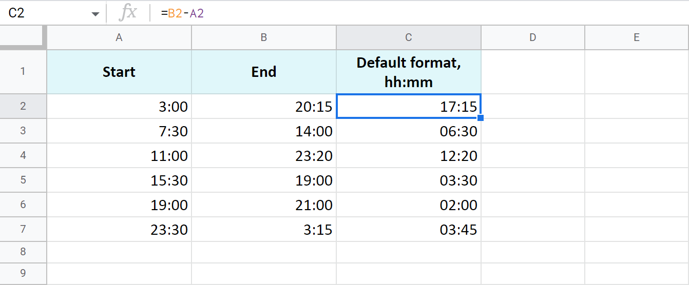
The time is formatted as "hh:mm" by default.
To get the results as hours only or as hours, minutes, and seconds, you need to apply a custom format with the corresponding time codes: h and hh:mm:ss. Google even offers a special number format for cases like this - Duration:
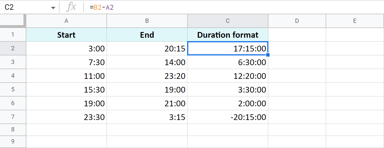
Tip. To apply the custom time format, go to Format > Number > Custom number format in your spreadsheet menu.
Example 2. Calculate time duration in Google Sheets using the TEXT function
Another trick to calculate the time duration in Google Sheets involves the TEXT function:
=TEXT(B2-A2,"h") - for hours
=TEXT(B2-A2,"h:mm") - for hours and minutes
=TEXT(B2-A2,"h:mm:ss") - for hours, minutes, and seconds
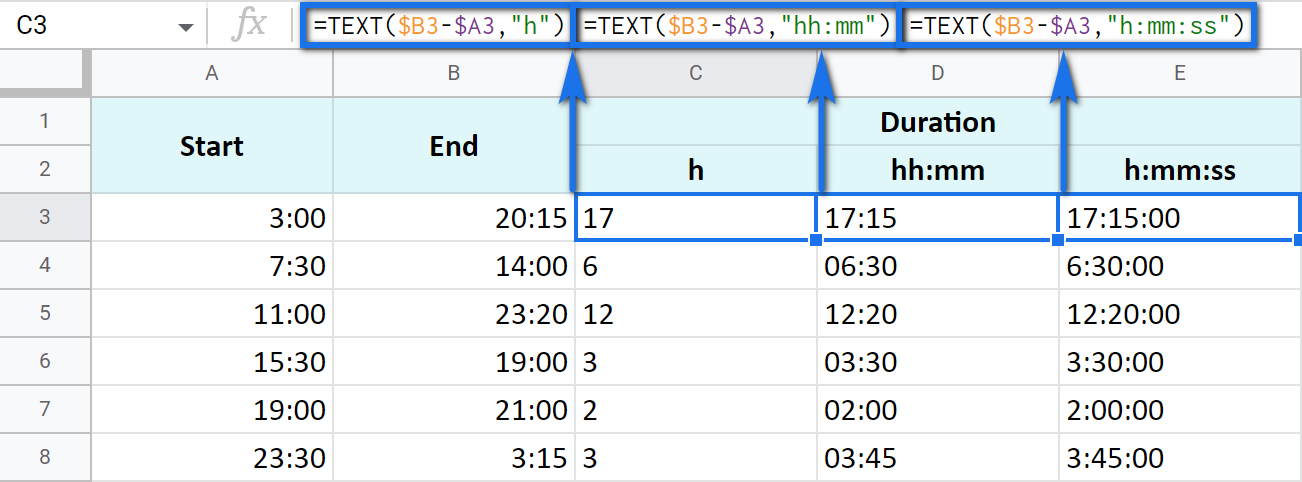
Note. See how the records are aligned to the left? Because the TEXT function always returns the results formatted as a text. This means these values cannot be used for further calculations.
Example 3. Time difference in hours, minutes, and seconds
You can track the time spent and get the result in one time unit disregarding other units. For example, count the number of only hours, only minutes, or only seconds.
Note. To ensure correct results, your cells should be formatted either as numbers or automatically: Format > Number > Number or Format > Number > Automatic.
-
To get the number of hours spent, subtract your start time from the end time and multiply the result by 24 (since there are 24 hours in one day):
=(End time - Start time) * 24You will get a time difference as a decimal:

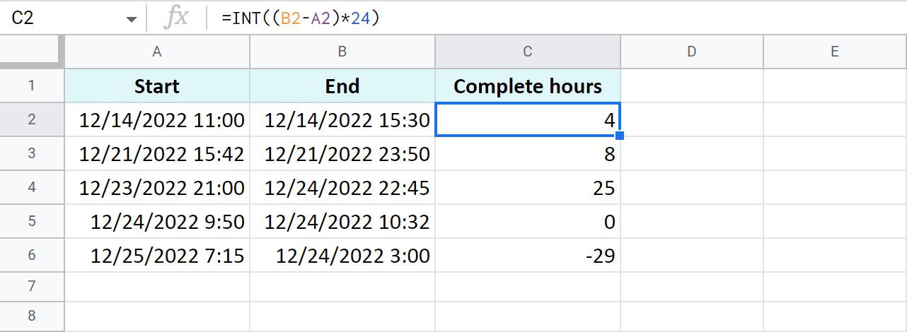
If the start time is greater than the end time, the formula will return a negative number, like in C5 in my example.
Tip. The INT function will let you see the number of complete hours spent since it rounds numbers down to the nearest integer:
-
To count minutes, subtract the start time from the end time and multiply whatever you get by 1,440 (since there are 1,440 minutes in one day):
=(End time - Start time) * 1440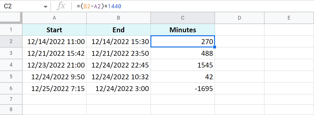
-
To find out how many seconds passed between two times, the drill is the same: subtract the start time from the end time and multiply the result by 86,400 (the number of seconds in a day):
=(End time - Start time) * 86400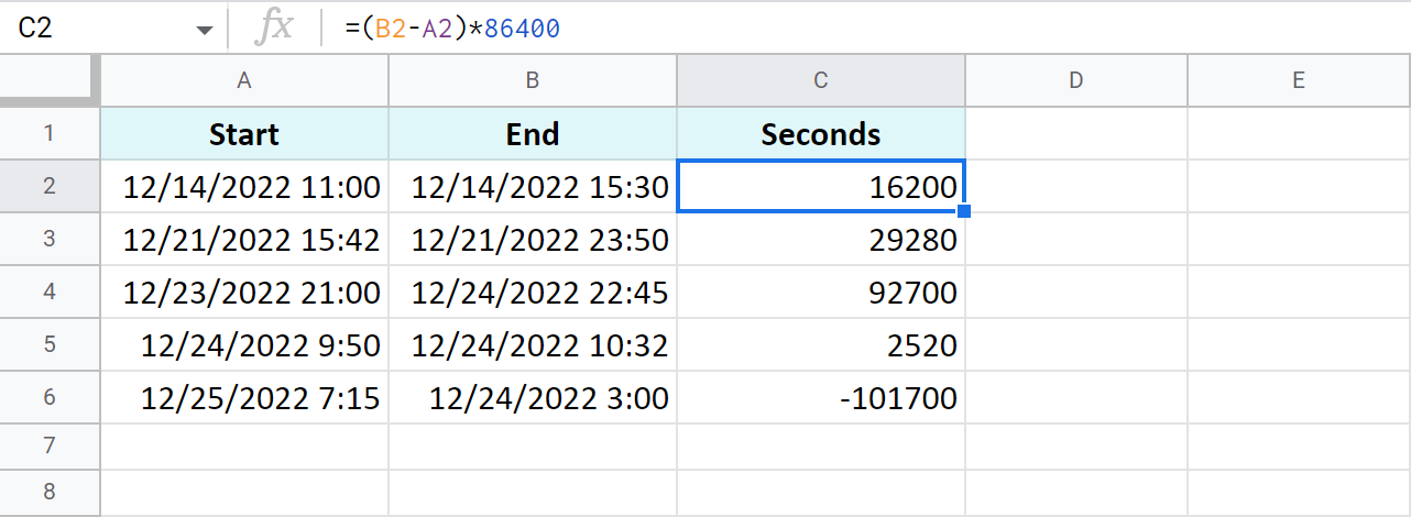
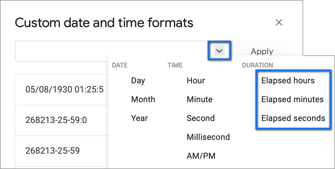
Tip. You can avoid multiplying in all these cases. Just subtract times first, and then apply elapsed time format from Format > Number > Custom date and time. If you click the down arrow to the right of the text field, you'll be able to choose between additional date and time units:
Example 4. Functions to get the time difference in a Google spreadsheet
As always, Google Sheets equips you with three particularly useful functions for this purpose.
Note. These functions work only within 24 hours and 60 minutes and seconds. If the time difference exceeds these limits, the formulas will return errors.
=HOUR(B2-A2)- to return hours only (without minutes and seconds)=MINUTE(B2-A2)- to return minutes only (without hours and seconds)=SECOND(B2-A2)- to return seconds only (without hours and minutes)

How to add and subtract time in Google Sheets: hours, minutes, or seconds
These operations can also be achieved with two techniques: one involves basic math calculations, another - functions. While the first way always works, the second one with functions works only when you add or subtract units less than 24 hours, or 60 minutes, or 60 seconds.
Add or subtract hours in Google Sheets
-
Add less than 24 hours:
=Start time + TIME(N hours, 0, 0)Here's how the formula looks on real data:
=A2+TIME(3,0,0)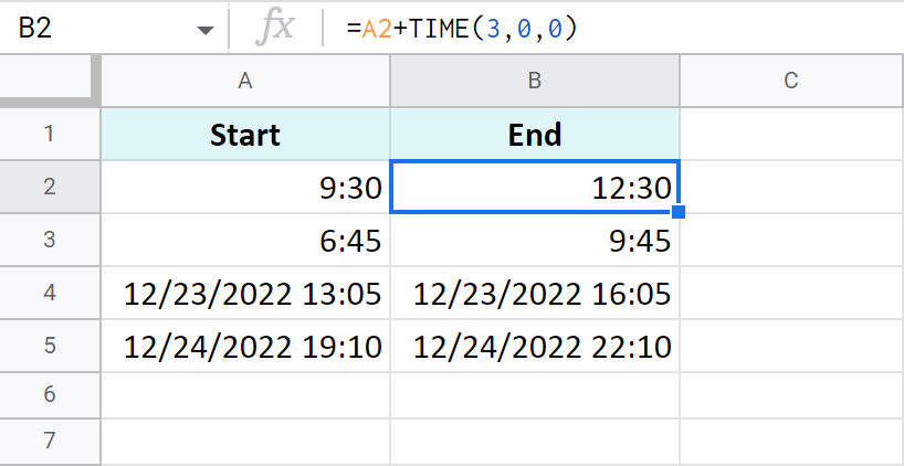
-
Add more than 24 hours:
=Start time + (N hours / 24)To add 27 hours to the time in A2, I use this formula:
=A2+(27/24)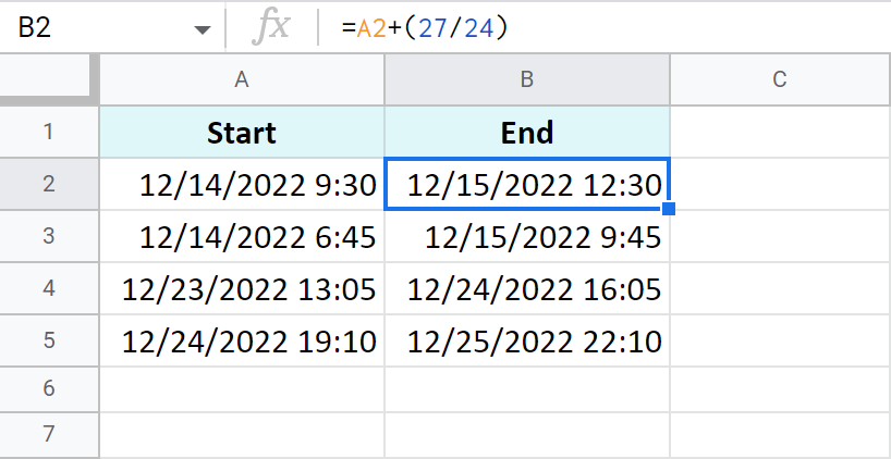
- To subtract 24 and more hours, use the formulas above as a basis but change the plus sign (+) to the minus sign (-). Here's what I've got:
=A2-TIME(3,0,0)- to subtract 3 hours=A2-(27/24)- to subtract 27 hours
Add or subtract minutes in Google Sheets
The principle of manipulating minutes is the same as with the hours.
-
There's the TIME function that adds and subtracts up to 60 minutes:
=Start time + TIME(0, N minutes, 0)If you are to add 40 minutes, you can do it like this:
=A2+TIME(0,40,0)If you are to subtract 20 minutes, here's the formula to use:
=A2-TIME(0,40,0)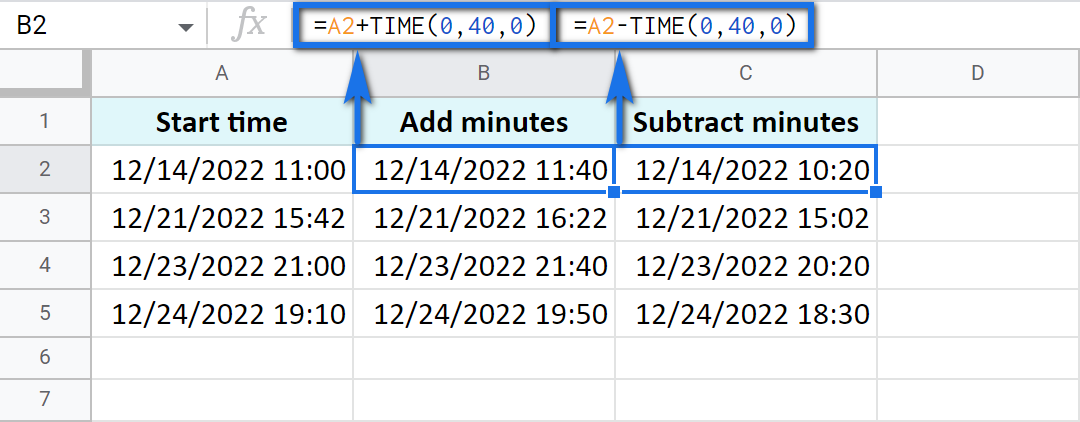
-
And there's a formula based on simple arithmetic to add and subtract over 60 minutes:
=Start time + (N minutes / 1440)Thus, here's how you add 120 minutes:
=A2+(120/1440)Put the minus instead of plus to subtract 120 minutes:
=A2-(120/1440)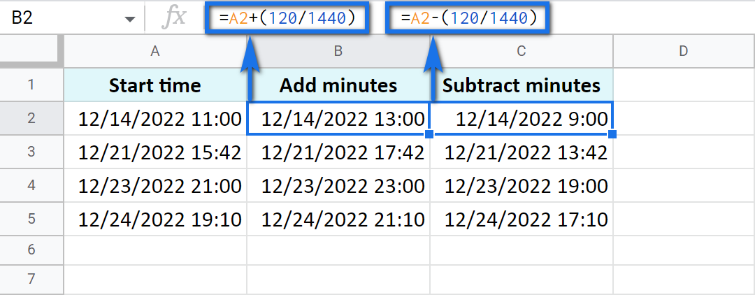
Add or subtract seconds in Google Sheets
Seconds in Google Sheets are calculated in the same manner as hours and minutes.
-
You can use the TIME function to add or subtract up to 60 seconds:
=Start time + TIME(0, 0, N seconds)For example, add 30 seconds:
=A2+TIME(0,0,30)Or subtract 30 seconds:
=A2-TIME(0,0,30) -
To calculate over 60 seconds, use simple maths:
=Start time + (N seconds / 86400)Add 700 seconds:
=A2+(700/86400)Or subtract 700 seconds:
=A2-(700/86400)
How to sum time in Google Sheets
To find the total time in your table in Google Sheets, you can use the SUM function. The trick here is to choose the correct format to display the result.
By default, the result will be formatted as Duration - hh:mm:ss
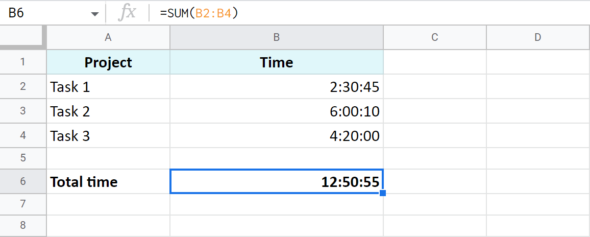
But most often the default time or duration format won't be enough, and you will need to come up with your own one.
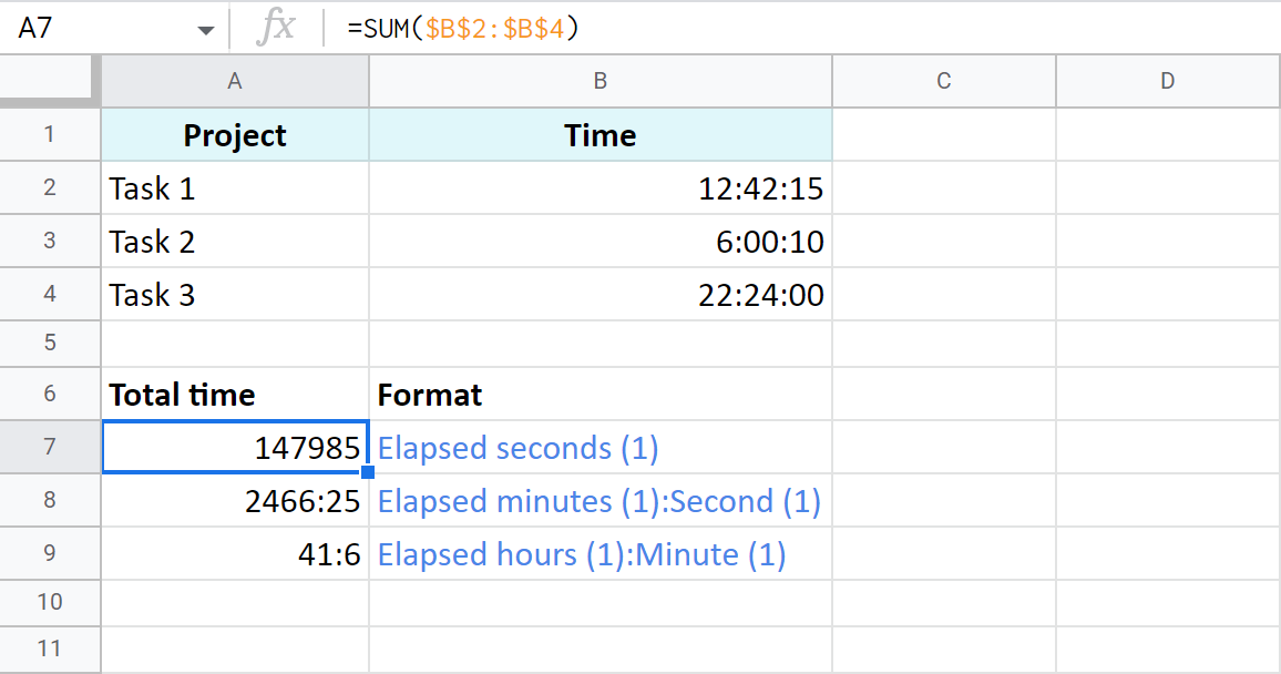
A7:A9 cells contain the same time value. They are just displayed differently. And you can actually perform calculations with them: subtract, sum, convert to decimal, etc.
Extract date and time from a full "date-time" record
Let's imagine that one cell in Google Sheets contains both, date and time. You want to set them apart: extract only the date to one cell and only time to another.
Split Date time using Number format
In order to display date or time in one cell on your screen or to print it, just select the original cell, go to Format > Number and choose Date or Time.
However, if you'd like to use these values for future calculations (subtract, sum, etc.), this won't be enough. If you don't see the time unit in a cell, it doesn't necessarily mean that it's absent, and vice versa.
So what do you do?
Split Date time using formulas
Google stores dates and time as numbers. For example, it sees the date 8/24/2017 11:40:03 as the number 42971,4861458. The integer part represents the date, the fractional - time. So, your task is down to separating integer from fractional.
- To extract date (integer part), use the ROUNDDOWN function in cell B2:
=ROUNDDOWN(A2,0)
The formula rounds the value down and casts the fractional part away.
-
To extract time, place the following subtraction formula into C2:
=A2-B2 -
Copy the results into the third row and apply Date format to B3 and Time format to C3:

Use the Split Date & Time add-on
You may be surprised but there's one special add-on for this job. It's really small and easy but its contribution to Google Sheets cannot be overstated.
Split Date & Time splits all Date time records in your entire column at once. You control the desired outcome with just 4 simple settings:
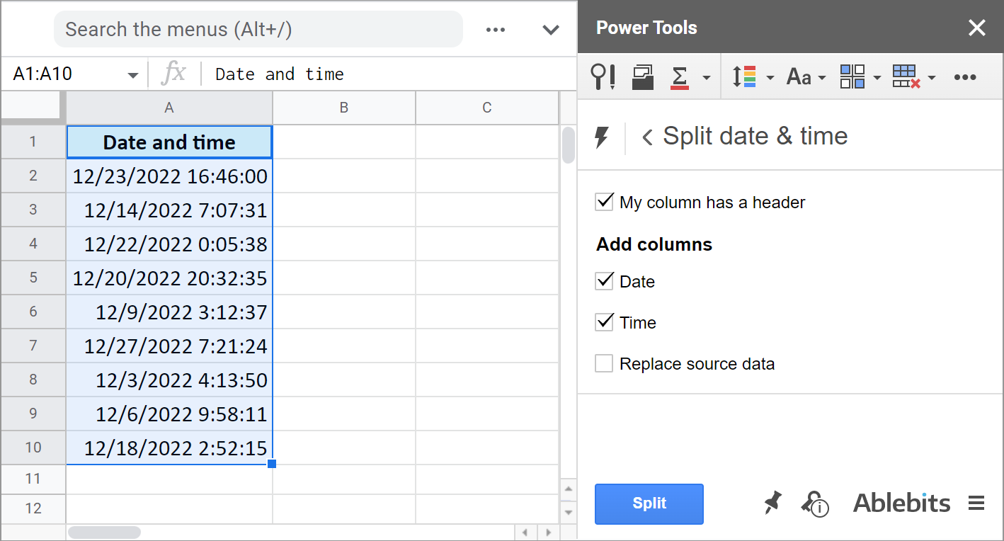
You tell the add-on:
- Whether there's a header row.
- If you want to get the Date unit.
- If you want to get the Time unit.
- And if you'd like to replace your original column with the new data.
It literally takes the burden of splitting date and time units off your shoulders:
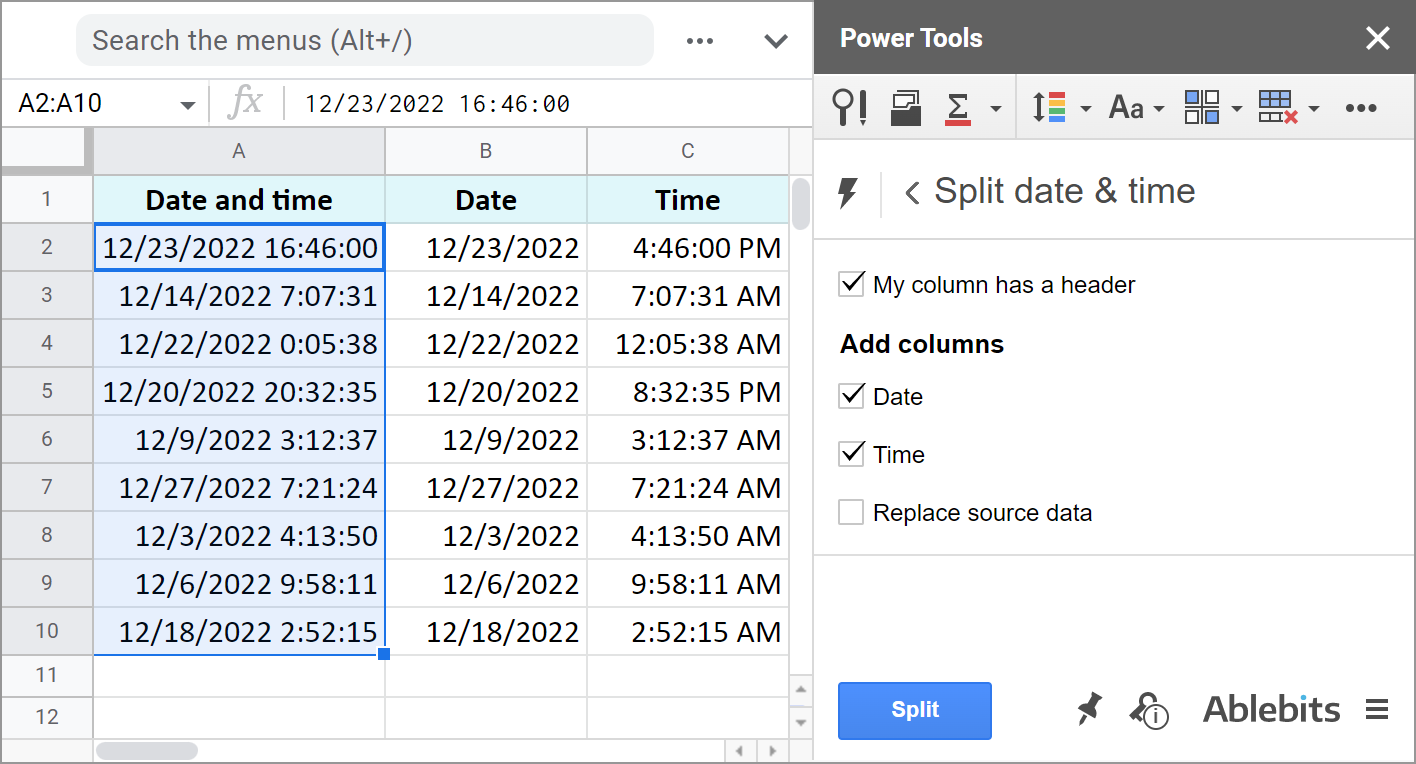
The add-on is part of the Power Tools collection so you will have more than 40 other useful add-ons at hand:
These are the ways to not only display date or time, but to separate them to different cells. And you can perform various calculations with these records now.
I hope these examples will help you solve your tasks when working with dates and time in Google Sheets.
Spreadsheet with formula examples
Calculating time in Google Sheets (make yourself a copy to practice)
 by
by 
393 comments
Hello,
I am having a problem adding and subtracting hour duration. Addition seems to be working correctly (6:30+2:00=8:30 8 hours 30 minutes). But I would like to subtract the total from 40 hours (40:00-8:30=31:30). Instead sheets is converting hours to days (when putting (40-31:30) in the cell it computes to 960:00-31:30=928:30). If I enter 40:00 - 31:30 I receive an error.
Hello Katie,
When you enter 40-31:30, Google Sheets treats those as numbers and can't count.
I'd advise you to put your durations in separate cells; then apply the duration format to them (Format > Number > Duration); and then use cell references to count =A2-B2. Everything will then work flawlessly.
Hey Natalia,
Thanks for taking the time to respond. The first 2 zeros are always just 00 but I'm guessing they're days? it is suppose to be hh:mm:ss. The data itself is copied from another source and even if I tried all sorts of format, it stays the same.
Hey Mac,
Thank you for the details.
Unfortunately, Google Sheets doesn't recognize values formatted as XX:XX:XX:XX as any types of dates. It automatically aligns them to the left and treats as text strings.
You need to remove those first zeros, and the records will then be automatically turned into Duration.
Btw, we have a tool that can help you remove chars by position quickly. It is free for 30 days and you can use it on your data and remove the first 3 chars (00:).
I've been trying to SUMIF the duration but always ends up with 0. After playing around I've found that because the data (Name and duration only, no start or end time) was in XX:XX:XX:XX format it doesn't work. If i remove the first 2 leading zeros, that's the only time the SUMIF or even SUM function would work. Any idea how to make this work?
Mac,
the duration format for Google Sheets is:
elapsed hours : elapsed minutes : elapsed seconds
What should another pair of numbers represent? Milliseconds?
Please go to Format > Number > More Formats > More date and time formats, and make sure you've set the correct format for your durations.
Can I ask how can you convert 3 mins 51 secs to 00:03:51 format? Thanks.
If your cell states "3 mins 51 secs", you won't be able to convert it. Since it contains text, Google will interpret it as a string.
But if you have 3:51 in a cell, custom number formats will do the trick. You can read more about them in this blog post.
Thanks.
Hi,
I've built a Google Sheet to track service/repair work on construction equipment by our shop technicians.
There are several steps in the operation process - 1) equipment arrives, 2) diagnostics, 3) labor quote by service dept., 4) parts quote by service, 5) full-quote sent to customer, 6) customer response, etc. We are date/time stamping each step of the process using this format (6/19/2019 0:00:00).
I built a column to calculate the duration between each step to help identify the stages of the process where we have the biggest opportunity to gain efficiencies (time). A sample formula I used for the calculation is - =ArrayFormula(IFERROR(if(Len(F3:F),(int(H3:H-F3:F)&"d "&text(H3:H-F3:F-int(H3:H-F3:F),"HH:MM:SS")),)))
While the duration formula above works great, I found that when I attempted to add an additional column of a target time frame (i.e. - 6 hours to complete for example); I could not use a comparative formula ( =if(I3>=J3,"X","√") ) because the duration calculation is in Text format.
Any thoughts? I'm trying to highlight work orders (conditional formatting) that are outside of target deadlines, so that managers spend more time focusing on the "jobs" that are underperforming.
Thanks!
Hi Kurt,
Since you use the TEXT function in your formula and such textual parts as &"d "&, the result will be turned into a text string. I'm afraid there's no way to make Google understand it as duration and compare with other time. I can only suggest you build a formula without using text parts in it.
Hi there!
Thank you so much for this helpful information.
Is it possible to calculate a sum of the total time formulas?
e.g.: (=TEXT($F3-$E3,"hh:mm")) + (=TEXT($F4-$E4,"hh:mm")) = (=SUM(G3:G33))
I have been trying the above to reach a sum but to no avail.
Thank you!
Lauren
Hi Lauren,
If I got your formula right, the TEXT function returns records as text and they cannot be used for calculations as is. You could try using VALUE in order to turn Text cells back to Time like this:
VALUE(TEXT((F3-E3),"HH:MM"))
but VALUE doesn't take ranges, so you'd have to do that for each cell within your range - G3:G33 - in order to create a formula:
=SUM(VALUE(TEXT((F3-E3),"HH:MM")),VALUE(TEXT((F4-E4),"HH:MM")),VALUE(...),...)
I'm trying to find a formula that converts duration in hr:min:sec format (e.g. 00:04:15) to total seconds in number format (255).
Any help greatly appreciated.
Hello Peter,
Please try the following:
=HOUR(A1)*3600+MINUTE(A1)*70+SECOND(A1)
how do i get the the total seconds for two cells. example start time is 6:44:56 am and end time 6:48:30 am?
Hello Bryan,
If you need to have both start and end time in seconds, use the formula from the comment you replied to. Just remember to use your own cell references.
If you need the time difference in seconds, first, find it by the example of the first paragraph, then apply the formula from the comment you replied to.
Is there a way to calculate the elapsed time for 2 different dates and times with a format of hours and minutes (hh:mm)?
Katrina,
Fist, subtract the start time from the end time. Then, select the results and go to Format > Number > More formats > More date and time formats. Set and apply the following:
Elapsed hours:Minute
Hope this helps.
How to calculate time only between working hours
Example employee started a task 2019-05-23 13:00 and finished 2019-05-28 10:00 it says 117hours but we are only open from 9 to 6 monday to friday is there way to only calculated hours between those time ?
Thanks !
Cedrik,
Let's assume your data looks the following way:
Where the opening time is in B1, closing time - in B2, the start task time is in B5, end task time in C5.
Here's the formula that should work:
=(NETWORKDAYS(B5,C5)-2)*(B2-B1)+(B2-MOD(B5,1))+(MOD(C5,1)-B1)
Newbie here! This is the formula I am using in a Google sheet to determine the time elapsed between opening a job ticket and completion. How do I make it account for work days? It's currently adding 2 days for jobs started Friday but completed on Monday.
=CONCATENATE(TEXT(FLOOR(L753-F753,1),"@")," Days",TEXT(L753-F753," h:mm"))
Hi Patty,
We've added NETWORKDAYS to your formula - this function is used to count the number of working days between two dates. As a result, we've got this:
=CONCATENATE(TEXT(NETWORKDAYS(F753,L753)-1,"@"),if((NETWORKDAYS(F753,L753)-1)=1," Day"," Days"),TEXT(L753-F753," h:mm"))
Please help me with this formula so it doesn't include weekends.
=ArrayFormula(IFERROR(if(Len(C2:C),(int(K2:K-C2:C)&"d "&text(K2:K-C2:C-int(K2:K-C2:C),"HH:MM:SS")),)))
Hello Lint,
I'm sorry but we need to see your data to be able to help. Please consider sharing an editable copy of your spreadsheet along with the formula with us (support@apps4gs.com). If you have confidential information there, you can replace it with some irrelevant data, just keep the format.
Note. We keep that Google account for file sharing only, please do not email there. Once you share the file, just confirm by replying here.
We'll look into it and try to help.
In the meantime, you can use our Multiple VLOOKUP Matches add-on for Google Sheets to pull the necessary data without the weekends first and then process it the way you need.
I noticed that when changing Duration to hours, day, etc... the Hours are always one day off. I notice this on your and on mine as well. Example: above you had 81:01:40 and it displayed 2 days, 1 hour, 40 minutes. It should be 3 days, 1 hour, 40 minutes.
Any idea why it automatically drops a day off?
thanks
Hi Robert,
Thank you for pointing that out.
We'll update this article with more correct calculations soon.
Hi,
I'm trying to create a sheet for hours worked with start and stop times. They way we usually calculate it, we enter the hours worked first, and have to add in the start and stop times later. If the employees always start and take lunch at the same time, how could I make a formula that will auto-populate the start and stop times for the amount of hours worked for a given day?
Ex: Start Stop Start Stop Hours
7:30 AM 12:00 PM 12:30 PM 4:30 PM 8
I would like to just be able to enter in "8" in the hours column, and have the start & stop times be calculated using a formula. Thank you!
Hi
These are probably dumb questions but here goes....
How would I calculate time elapsed by days on a project I'm tracking.
Ex: Task 1 is supposed to start 1/23/18 but it did not start until 1/26/18
I also am using conditional formatting in a status column.
Is it possible to just have Task column, Start date column, Days Delayed column and Status column.
Hi Lauren,
You can calculate the time difference between dates and have it returned in days:
=DATEDIF(A2,B2,"D")
As for your second question, could you please specify what you mean in detail?
Halima’s slept at 2200h if she woke up at 0600h for how long had she slept.
Hi thank you for the above time calculation.
There is one more help I need about the above formula. Is there a way to know the time spent on a particular task submitted per employee.
Example : An employee used google form to submit a completed task. That showed 8/10/2018 6:30:00 timestamp, then claimed a new task which ended at 8/10/2018 7:15:00, then claimed another task which ended at 8/10/2018 7:35:00. Employees let’s say are required to complete 3 task per hour. In a situation where by one has more than hundreds of people using the form to submit their task completion per hour in one google tracker . What is the easiest way to calculate the hr spent by each employee and the completed task per hour. 2 is there a way to add a formula on a separate column that auto calculate hours spent by each employee when 3task is completed. ? The logic here is I would like to know the most product employee in an hour thanks.
Looking to set a series of times based upon a single "operator entered START time" and about 10 subsequent times where I know the number of minutes between each step.
It would be quite possible these would go over midnight to the next day.
Example: Start time = 11:00 AM
Step 1 [15 min] = 11:15 AM
Step 2 [20 min] = 11:35 AM
Step 3 [4 hours] = 3:35 PM
Thanks!
I'm looking for the same!
I'd like input the event start time and have it populate the cells with a list of times other coordinated events will be happening
Hi, I'm trying to sort out how to sum time for a time trial event on a racing game. There are several weeks being added together for a total combined time of all events. The issue I'm having is Sheets is rounding the time up. I need it to show exact times, so if a lap time is 1 minute 33 seconds and .742 so, 0:01:33.742, I need it to show that time in the cell, and to represent that time in the total time cell, which I've used the sum function for. Drivers' times are often too close for them to be rounded up.
Any help appreciated! Thanks!
Dave:
Have you tried to use this in the Custom section of the Format Cells? mm:ss.000
Hey!
Thanks for a super interesting topic. I'm trying to build a countdown displaying Days, Hours and Minutes and yours is the only subject I can find on the matter.
Though I have some major problems getting it to work correctly and was wondering: Would you mind sharing your Sheet for us slow people to have a poke at?
Thanks in advance and thanks for a super post!
//Ola
HI, When the "duration, h" column is added to get a total hours the formula SUM(E3:E100) returns less than 24 hours. It restarts the summation each time it hits 24 hours. So if the total hours worked is 53 hours and 45 minutes, the return is 5:45 which is incorrect. How can I correct that?
G:
How is the cell duration h formatted?
The issue may be one of formatting the cell the way you want it to display.
Solved the same problem by changing the number format in the sum cell to [h]:mm:ss instead of h:mm:ss
Actually the above was in onedrive excel, not google sheets
I also need to fix this. Trying to convert 2 week pay period that is reported in hours 72:30:00 into a decimal of 72.5 hours.
Hello Travis,
You need to multiply a cell with that duration by 24 and format the resulting cell as a number.
I mention decimals in the following section: "Example 3. Time difference in hours, minutes, and seconds.". It's in the first part of the blog post, please take a look.
Thank you! This just saved me so much time!
Get it? Time? Like this article?
Seeya guys, gonna off myself.