This tutorial explains the basics of Excel structured references and shares some tricks on using them in real-life formulas.
One of the most useful features of Excel tables are structured references. When you have just stumbled upon a special syntax for referencing tables, it may look boring and confusing, but after experimenting a bit you will surely see how useful and cool this feature is.
Excel structured reference
A structured reference, or table reference, is special way for referencing tables and their parts that uses a combination of table and column names instead of cell addresses.
This special syntax is required because Excel tables (vs. ranges) are very powerful and resilient, and normal cell references cannot adjust dynamically as data is added or removed from a table.
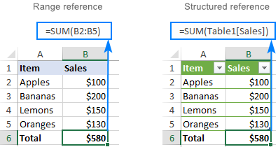
For example, to sum the values in cells B2:B5, you use the SUM function with a usual range reference:
=SUM(B2:B5)
To add up the numbers in the "Sales" column of Table1, you use a structured reference:
=SUM(Table1[Sales])
Key features of structured references
Compared to standard cell references, table references have a number of advanced features.
Easily created
To add structured references to your formula, you simply select the table cells you want to refer to. The knowledge of a special syntax is not required.
Resilient and automatically updated
When you rename a column, references are automatically updated with the new name, and a formula does not break. Moreover, as you add new rows to the table, they are immediately included in the existing references, and the formulas calculate the full set of data.
So, whatever manipulations you do with your Excel tables, you don't have to worry about updating the structured references.
Can be used inside and outside a table
Structured references can be used in formulas both inside and outside an Excel table, which makes locating tables in large workbooks easier.
Formula auto-fill (calculated columns)
To perform the same calculation in each table row, it is enough to enter a formula in just one cell. All other cells in that column are filled automatically.
How to create a structured reference in Excel
Making a structured reference in Excel is very easy and intuitive.
If you are working with a range, convert it to an Excel table first. For this, select all the data and press Ctrl + T. For more information, please see How to create a table in Excel.
To create a structured reference, this is what you need to do:
- Start typing a formula as usual, beginning with the equality sign (=).
- When it comes to the first reference, select the corresponding cell or range of cells in your table. Excel will pick up the column name(s) and create an appropriate structured reference for you automatically.
- Type the closing parenthesis and press Enter. If the formula is created inside the table, Excel automatically fills the entire column with the same formula.
As an example, let's add up the sales numbers for 3 months in each row of our sample table, named Sales. For this, we type =SUM( in E2, select B2:D2, type the closing parenthesis, and press Enter:
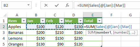
As the result, the whole column E is auto-filled with this formula:
=SUM(Sales[@[Jan]:[Mar]])
Though the formula is the same, the data is calculated in each row individually. To understand the inner mechanics, please take a look at the table reference syntax.
If you are entering a formula outside the table, and that formula requires only a range of cells, a faster way to make a structured reference is this:
- After the opening parenthesis, start typing the table name. As you type the first letter, Excel will show all matching names. If necessary, type a couple more letters to narrow down the list.
- Use the arrow keys to select the table name in the list.
- Double-click the selected name or press the Tab key to add it to your formula.
- Type the closing parenthesis and press Enter.
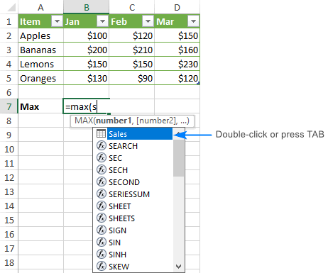
For example, to find the largest number in our sample table, we start typing the MAX formula, after the opening parenthesis type "s", select the Sales table in the list, and press Tab or double-click the name.
As the result, we have this formula:
=MAX(Sales)
Structured reference syntax
As already mentioned, you do not need to know the syntax of structured references to include them in your formulas, however it will help you understand what each formula is actually doing.
Usually, a structured reference is represented by a string that begins with a table name and ends with a column specifier.
As an example, let's break down the following formula that adds up the totals of the South and North columns in the table named Regions:

The reference includes three components:
- Table name
- Item specifier
- Column specifiers
To see what cells are actually calculated, select the formula cell and click anywhere in the formula bar. Excel will highlight the referenced table cells:

Table name
The table name references only the table data, without header row or total rows. It can be a default table name like Table1 or a custom name like Regions. To give a custom name to your table, carry out these steps.
If your formula is located within the table it refers to, the table name is usually omitted because it is implied.
Column specifier
Column specifier references the data in the corresponding column, without the header row and total row. A column specifier is represented by the column name enclosed in brackets, e.g. [South].
To refer to more than one contiguous columns, use the range operator like [[South]:[East]].
Item specifier
To refer to specific parts of a table, you can use any of the following specifiers.
| Item specifier | Refers to |
| [#All] | The entire table, including table data, column headers and total row. |
| [#Data] | The data rows. |
| [#Headers] | The header row (column headers). |
| [#Totals] | The total row. If there's no total row, it returns null. |
| [@Column_Name] | The current row, i.e. the same row as the formula. |
Please notice that the pound sign (#) is used with all the item specifiers, except the current row. To refer to the cells in the same row where you enter the formula, Excel uses the @ character followed by the column name.
For example, to add numbers in the South and West columns of the current row, you'd use this formula:
=SUM(Regions[@South], Regions[@West])
If the column names contain spaces, punctuation marks or special characters, an additional set of brackets around the column name will appear:
=SUM(Regions[@[South sales]], Regions[@[West sales]])
Structured reference operators
The following operators allow you to combine different specifiers and add even more flexibility to your structured references.
Range operator (colon)
As with normal range references, you use a colon (:) to refer to two or more adjacent columns in a table.
For example, the below formula adds up the numbers in all the columns between South and East.
=SUM(Regions[[South]:[East]])
Union operator (comma)
To refer to non-adjacent columns, separate the column specifiers with commas.
For instance, here's how you can sum the data rows in the South and West columns.
=SUM(Regions[South], Regions[West])
Intersection operator (space)
It is used to refer to a cell at the intersection of a specific row and column.
For example, to return a value at the intersection of the Total row and West column, use this reference:
=Regions[#Totals] Regions[[#All],[West]]
Please notice that the [#All] specifier is required in this case because the column specifier does not include the total row. Without it, the formula would return #NULL!.
Table reference syntax rules
To edit or make structured references manually, please follow these guidelines:
1. Enclose specifiers in brackets
All column and special item specifiers must be enclosed in [square brackets].
A specifier that contains other specifiers should be wrapped in outer brackets. For example, Regions[[South]:[East]].
2. Separate inner specifiers with commas
If a specifier contains two or more inner specifiers, those inner specifiers need to be separated with commas.
For example, to return the header of the South column, you type a comma in between [#Headers] and [South] and enclose this whole construction in an additional set of brackets:
=Regions[[#Headers],[South]]
3. Do not use quotation marks around column headers
In table references, column headers don't require quotes whether they are text, numbers or dates.
4. Use a single quotation mark for some special characters in column headers
In structured references, some characters such as left and right brackets, pound sign (#) and single quotation mark (') have special meaning. If any of the above characters is included in a column header, a single quotation mark needs to be used before that character in a column specifier.
For example, for the column header "Item #", the specifier is [Item '#].
5. Use spaces to make structured references more readable
To improve the readability of your table references, you can insert spaces in-between specifiers. Normally, it is considered a good practice to use spaces after commas. For example:
=AVERAGE(Regions[South], Regions[West], Regions[North])
Excel table references - formula examples
To gain more understanding about structured references in Excel, let's go over a few more formula examples. We'll try to keep them simple, meaningful and useful.
Find the number of rows and columns in an Excel table
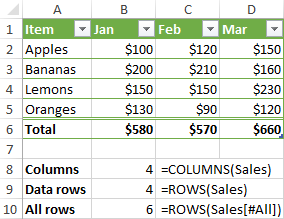
To get the total columns and rows count, use the COLUMNS and ROWS functions, which only require the table name:
For example, to find the number of columns and data rows in the table named Sales, use these formulas:
=COLUMNS(Sales)
=ROWS(Sales)
To include the header and total rows in the count, use the [#ALL] specifier:
=ROWS(Sales[#All])
The below screenshot shows all the formulas in action:
Count blanks and non-blanks in a column
When counting something in a specific column, be sure to output the result outside the table, otherwise you might end up with circular references and wrong results.
To count blanks in a column, use the COUNTBLANK function. To count non-blank cells in a column, utilize the COUNTA function.
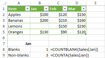
For example, to find out how many cells in the Jan column are empty and how many contain data, use these formulas:
Blanks:
=COUNTBLANK(Sales[Jan])
Non-blanks:
=COUNTA(Sales[Jan])
To count non-blank cells in visible rows in a filtered table, use the SUBTOTAL function with function_num set to 103:
=SUBTOTAL(103,Sales[Jan])
Sum in an Excel table
The fastest way to add up numbers in an Excel table is to enable the Total Row option. To do this, right click any cell within the table, point to Table, and click Totals Row. The total row will appear at the end of your table straight away.
Sometimes Excel may assume you want to total only the last column and leaves other cells in the Total row blank. To fix this, select an empty cell in the Total row, click the arrow that appears next to the cell, and then select the SUM function in the list:
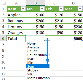
This will insert a SUBTOTAL formula that sums values only in visible rows, ignoring filtered-out rows:
=SUBTOTAL(109,[Jan])
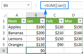
Please note that this formula works only in the Total row. If you try to manually insert it in a data row, this would create a circular reference and return 0 as the result. A SUM formula with a structured reference won't work either for the same reason:
So, if you want the totals inside the table, you need to either enable the Total row or use a normal range reference such as:
=SUM(B2:B5)
Outside the table, the SUM formula with a structured reference works just fine:
=SUM(Sales[Jan])
Please note that unlike SUBTOTAL, the SUM function adds up values in all the rows, visible and hidden.
Relative and absolute structured references in Excel
By default, Excel structured references behave in the following way:
- Multiple column references are absolute and do not change when formulas are copied.
- Single column references are relative and change when dragged across columns. When copied/pasted via a corresponding command or shortcuts (Ctrl+C and Ctrl+V), they do not change.
In situations when you need a combination of relative and absolute table references, there is no way to copy the formula and keep table references correct. Dragging the formula will change the references to single columns, and copy/pasting shortcuts will make all the references static. But there are a couple of simple tricks to get around!
Absolute structured reference to single column
To make a single column reference absolute, repeat the column name to formally turn it into a range reference.
Relative column reference (default)
table[column]
Absolute column reference
table[[column]:[column]]
To make an absolute reference for the current row, prefix the column identifier by the @ symbol:
table[@[column]:[column]]
To see how relative and absolute table references work in practice, please consider the following example.
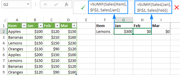
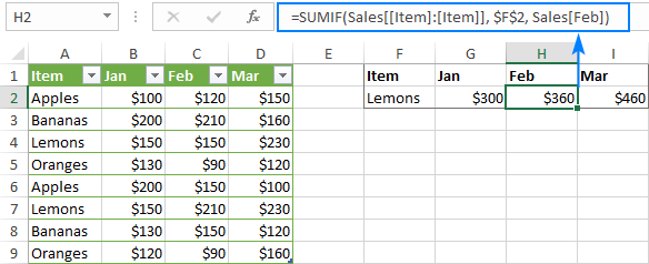
Supposing you want to add up the sales numbers for a specific product for 3 months. For this, we enter the target product name in some cell (F2 in our case) and use the SUMIF function to get the total of Jan sales:
=SUMIF(Sales[Item], $F$2, Sales[Jan])
The problem is that when we drag the formula to the right to calculate the totals for the other two months, the [Item] reference changes, and the formula breaks:
To fix this, make the [Item] reference absolute, but keep [Jan] relative:
=SUMIF(Sales[[Item]:[Item]], $F$2, Sales[Jan])
Now, you can drag the modified formula to other columns and it works perfectly:
Relative structured reference to multiple columns
In Excel tables, structured references to several columns are absolute by their nature and remain unchanged when copied to other cells.
To me, this behavior is very reasonable. But if you need to make a structured range reference relative, prefix each column specifier with the table name and remove the outer square brackets as shown below.
Absolute range reference (default)
table[[column1]:[column2]]
Relative range reference
table[column1]:table[column2]
To refer to the current row inside the table, use the @ symbol:
[@column1]:[@column2]
For example, the below formula with an absolute structured reference adds up the numbers in the current row of the Jan and Feb columns. When copied to another column, it will still sum Jan and Feb.
=SUM(Sales[@[Jan]:[Feb]])
In case you want the reference to change based on a relative position of the column where the formula is copied, make it relative:
=SUM(Sales[@Jan]:Sales[@Feb])
Please notice the formula transformation in column F (the table name is omitted because the formula is inside the table):

That's how you make table references in Excel. To have a closer look at the examples discussed in this tutorial, feel free to download our sample workbook to Excel Structured Reference. I thank you for reading and hope to see you on our blog next week.
 by
by
54 comments
"If your formula is located within the table it refers to, the table name is usually omitted because it is implied."
Please give an example, that is exactly what I need and I cannot find a way to do it. Instead of a table name (e.g., "Table38"), I need a way to say "this.table" - regardless of the name of the table.
Hello John!
I hope you have studied the recommendations in the tutorial above. If I understand your task correctly, here is a formula example:
=[@Quantity]*[@Price]
Hi! In Excel tables, the reference to the columns in the table is absolute and cannot be changed automatically when you copy a formula.
OK Alexander, thanks for the reply. I thought as much that there doesn't seem to be any solution.
Some time ago, I had set up a workaround for this issue... a UDF that gets the table name, and a macro that
(1) uses the value from the UDF ... and
(2) concatenates the desired table + column reference to create the formula for the other column(s).
It helps to reduce the editing time and manual errors when I have to do this for many columns in many tables.
Why don’t use indirect function to evaluate the dynamic part.
=inderect(“SUBTOTAL(3,Table1[“ & B1 & ”])”)
sorry by the previos comment, the next solution will work to solve your problem.
=SUBTOTAL(109,INDIRECT("tableName["&C9&"]"))
in just few words we should evaluate the dynamic part, which is the structure reference.
let me know if this solution works for you.
thanks.
I know I can use row() to get the row of the spreadsheet I'm in but is there a way to return the current row of the table itself? Or to at least get the location the table starts at so i can subtract it from row()?
I've got a table that looks like this:
Date Item 1 Item 2 Daily Total
1 5/4/2024 1 2 1
2 5/5/2024 3 1 5
3 5/5/2024 2 1 5
4 5/6/2024 3 2 3
If there are 2 rows with data for the same date, I'd like to keep the individual item counts, but just show the total in one line, like this:
Date Item 1 Item 2 Daily Total
1 5/4/2024 1 2 1
2 5/5/2024 3 1 5
3 5/5/2024 2 1
4 5/6/2024 3 2 3
Is there a way to do that easily?
Hi! If my understanding is correct, use COUNTIF counting in the IF formula to display the number of values only in the row where the value first appears. Try this formula:
=IF(COUNTIF($A$1:A1,A1)=1, COUNTIF($A$1:$A$100,A1), "")
Is there a way to reference a single cell within a named table based on either positioning criteria or the name/value of the column and row?
I have an table of offsets I am trying to apply to values within multiple other tables in a more robust, repeatable manner.
Using the example above, imagine that I had a sales table that is filled with regular sales data, but I have another table that represents income from other sources. If I wanted to total each cell individually (and their row numbers did not match), can I do that?
I am envisioning something like =Sales[Apples,Jan]+OtherInc[Apples,Jan], but that doesn't work (assuming the Sales and OtherInc tables do not use the same rows).
Hello!
You can combine two tables using the Combine Sheets tool and then calculate totals in that table. You can also use the Consolidate Sheets tool. Consolidate Sheets tool can summarize your data by column headers, row headers, or position in a table. It is available as a part of our Ultimate Suite for Excel that you can install in a trial mode and check how it works for free.
You can also use the SUMIFS formula to calculate the sum of the conditions in each table and then sum them.
I hope I answered your question. If something is still unclear, please feel free to ask.
Вы можете объединить две таблицы в одну и затем подсчитывать в ней итоги. Для этого можно использовать Combine Sheets tool. Вы можете использовать Consolidate Sheets tool, чтобы в новойТакже вы можете подсчитывать сумму по условию отдельно в каждой таблице при помощи формулы SUMIFS.
Does anyone know if this is possible?
Originally the formula was =COUNTIFS($A$2:A2,A2,$B$2,B2,B2)=1 - but whenever I delete rows, the top formula will be updated to the number of rows that were there before deletion because it's absolute mixed with relative. I can't make the other parts of the countifs absolute or the formula doesn't work. I wanted to see if doing it in table ref format would stop this.
I wanted to recreate it with the table refs but can't seem to do it. Thanks!
Hi! Your formula is written with an error and can't work. I recommend reading the instructions: Excel COUNTIFS and COUNTIF with multiple AND / OR criteria.
If the formula contains an absolute reference to row 2 ($A$2) and you delete rows 1 and 2, the formula will return error #REF!
Hello,
My structured reference formula refers to a table that is in another workbook. If I close this workbook the formula gives the "#REF!" result. How can I avoid that ?
Best regards,
Loïc.
Hi!
An Excel reference to another workbook works only when that workbook is open.
You can get data from a closed workbook only with VBA.
Hi,
Similar question to above.
Is there a way to automatically convert a formula containing cell references to structured references?
I have an existing file with sumifs formulas referencing a range in another tab and now what to delete some rows in the range but this results in the sumifs formulas being invalid as the cell references don't update.
So I have converted the range to a Table.
Can I automatically change the sumifs formulas to use the structured reference in the newly created table as opposed to the existing cell references?
Many thanks,
Patricia
Hello!
When you convert a range to a table, Excel does not automatically change the cell references in that range to the appropriate structured references.
To change part of the formula automatically, you can use the Excel Find & Select tool. (Look in: Fofmulas).
I hope it’ll be helpful.
I have calculations about a range of a table fSalesAn[Quantity], how can I receive the Quantity field, in text, without evoking fSalesAn[[#Headers];[Quantity]
Hello!
If I understood the problem correctly, you can use a regular cell reference. For example, =B1
Hi,
I am having a really tough time finding a solution for using greater and less than signs in combination with structured references. I have a specification table, that I am trying to call to so that I can count how many data points fall within a specified range. Currently, my formula looks like this:
=(COUNTIFS(Master!$B$2:$B$1000,Table1[@Brand],Master!$C$2:$C$1000,Table1[@Flavor],Master!$E$2:$E$1000,Table1[@[Month '#]],Master!$L$2:$L$1000,">[Specifications[Lower Limit]]",Master!$L$2:$L$1000,"<[Specifications[Upper Limit]]"))
Excel will not recognize the structured reference within quotations, is there another way to code the last two criteria of this formula?
Hello!
Please try the following formula:
=(COUNTIFS(Master!$B$2:$B$1000,Table1[@Brand],Master!$C$2:$C$1000,Table1[@Flavor], Master!$E$2:$E$1000,Table1[@[Month ‘#]], Master!$L$2:$L$1000,">"&[Specifications[Lower Limit]]”, Master!$L$2:$L$1000,"<"&[Specifications[Upper Limit]]"))
Please check out this article to learn how to use cell references in COUNTIFS formulas.
How do I make this dynamic with filtering? assume there is a date column i want to apply filters to. and the other columns are in a sum if formula.
ex. dates 1/1/21-1/1/22
Outside of the table i have a list of names each gets a formula like =SUMIF(Table3[Name],$A$300(there is a name here),Table3[Sales])
if I apply a filter to the date the table updates (hides non applicable data) but the value of the formula does not update.
Hello!
The SUMIF function counts the data in the hidden rows. If you use the Excel filter, I recommend paying attention to the SUBTOTAL function. She knows how to ignore hidden data. Or you can use the FILTER function to filter the data and then use SUMIF with that data.
I hope it’ll be helpful.
Hi
is there any way to reference in this formula =SUM(Sales[Jan]), the value between brackets to a cell value. I mean like this =SUM(Sales[a1]) where the value of A1 = Jan.
or in the floowing formula
index(Sales;SECUENCE(ROWS(SALES));{1\3\5}) VS index(Sales;SECUENCE(ROWS(SALES));{A1}), where A1 value = 1/3/5
Hello!
Please use the formula below to solve your task:
=SUM(INDIRECT("SALES["&A1&"]"))
See this guide for more information: Excel INDIRECT function - basic uses and formula examples.
I want a cells on another sheet to repeat the same values of a range of a table
Sheet 1 table which I wish to reference begins at row 2 because of headers
The sheet 2 table begins at row 4.
When I use =table[column] or =table[@column] in the cell of row 4 of the sheet 2 table it returns the value of sheet 1 row 4 and not the first row of the table (row 2 value)
Is there any way to use structured references but have them begin at the first row of the table being referred to and not the row from the reference table which corresponds to the cell which the equation was typed?
Hello!
Earlier in this article, it was said that the @ sign denotes an absolute reference to a cell in a column.
Table1[Column2] reference returns the entire column.
Table1[@Column2] reference returns one cell that corresponds to the line number in which the formula is written.
My apologies I should have been a bit more clear.
I have a table which has column where I want the exact same data to appear in another column but in a different table.
Table 1 Column 1 begins at row 2 because of headers
Table 2 Column 1 begins at row 4 because of headers
I put these functions into row 4 of column 1 in table 2
Table1[Column1] returns spill since it is a table
Table1[@Column1] returns the value at Row 4 of column 1 in table 2
Is there a way to reference Table 1[@column1] - 2 rows location?
Thank you
Hi!
Unfortunately, I have no solution to your question.
Great article, articulating this expression.
Keep it up!
I agree; thank you for this information and all the great replies to people's questions.
Thank you for the explanation. I am thinking how we can use the column name dynamically.
For example I have a table which have monthly purchases(January, February, etc. like month names are headers) . I don't have total column, but instead I have a cell below the table (not in the table reference) and I need to find the current month purchase total.
If current month is January, I need to update the total of January column. My table name is tblPurchase.
I can find the current month column name using MATCH formula like below
=CONCAT("tblPurchase[", TEXT(TODAY(), "mmmm"), "]")
But how can I use this column name as a reference? Assumed that A5 is the result cell of the above formula.
=SUBTOTAL(9, A5)
It returns 0 only. Can anyone help me
Hello!
Create a named range (for example, "March").
You can find the sum of the values from this named range using the formula
=SUM(INDIRECT(TEXT("03/01/2021","mmmm")))
You can learn more about named ranges in Excel in this article on our blog.
If this is not what you wanted, please describe the problem in more detail.
One additional nuanced scenario is if the column name is a number:
For example, when making a relative structured reference to multiple columns within the current row.
The above example works fine:
=SUM(Sales[@Jan]:Sales[@Feb])
...unless the column names are a number
Substituting
Jan = 2021.01
Feb = 2021.02
=SUM(Sales[@2021.01]:Sales[@2021.02]) *** This will not work!
An additional set of brackets around the column name is required:
=SUM(Sales[@[2021.01]]:Sales[@[2021.02]]) *** This works!
Hi Marty,
Thank you for your comment.
More precisely, that additional set of brackets is required because of the dot. If the columns names were integers, extra brackets wouldn't be needed.
The general rule is this: if the column names contain spaces, punctuation marks or special characters, an additional set of brackets around the column name should be added.
Again, thank you for this observation! We've added this information to the article.
Is there a way to convert a formula containing 'old-style' cell references to structured references. I have a set of formulas that reference a range I have converted into a table. Now I have to manually adjust $A3 to [@[Client ID]] in the formulas. It would be great if this could be done across a range of columns automatically similar to Insert > Name > Apply when using Named Ranges. Can it be done?
I have this same question, but I want to just show cell references because it is very difficult for me to read the names and figure it out as a formula but I would like to keep it as a table.
Joining 2 columns in a table. A number value in column A joined to a Date value in column B to form a text value in column C using formula C=A&" - "&month(B)
Tables converts this formula to
=[@Number]&" - "&MONTH([@[DATE]])
Sample;
65 Nov 26, 2020 65 - 11
66 Dec 07,2020 66 - 12
Is there a way to format the month portion only in column C so it displays as Nov and Dec...
Desired;
65 Nov 26, 2020 65 - Nov
66 Dec 07, 2020 66 - Dec
Hello!
If I understand your task correctly, the following formula should work for you:
=[@Number]&” – “&TEXT([@[DATE]],"mmmm")
You can read more about the TEXT function in the above linked article.
Totally impressed with all the great stuff that comes out of Ablebits. This is no exception. The problem is, and I hate to say this, I simply don't have the time or inclination to relearn a whole new way of writing and executing this new way of creating formulas and all the rules and exceptions involved. I am an old timer that learned spreadsheets on SuperCalc, 123 and Lotus then finally Microsoft came up with what I consider to be the last word in what I need for my fairly simple calcuations having to do with my stock day trading.
Sadly, a few years back, I decided to create a sophisticated Workbook whereby I created a primary worksheet comprised of 365 pivot tables for each day of the year. Each table has all my stock positions broke down into specific lots and and from that, I keep running totals of all kinds of statistical data I created with standard formulas. The workbook has all kinds of worksheets crammed with statistical data that I reference and use in the primary worksheet.
So, one day, I fiddled with one of the options for naming thinking that the use of the header names instead of standard cell references would make things easier. From that day on, Structured references began creeping into my formulas as I added things. I had no idea it would grow to be such a problem. It especially became prevalent when I imported CSV files and created new pivot tables in other worksheets. I also have a lot of worksheets in this workbook with long sophisticated names that I have to pull data from. Column Header names were also long but by making them that way, I knew precisely where to go to extract data. I learned to read my formulas fluently even with these setbacks and move around quickly and precisely over a period of time. Now, I am constantly having to physically remove structured names as they keep popping up like burnt popcorn and rewrite the formulas all over again. I finally found out how to get back into the proper location to turn off table names in formulas, but I have not found any way to force excel to convert all the structured names back to the good old Column, Row nomenclature and I either cannot figure out the proper way to phrase the proper question, perhaps there is no way to easily fix this but I really would like to purge all the structured references without having to start over again after all these years.
Sorry for the long winded explanation but I am hoping one of you fine people can help me with suggestions on how to proceed, or steer me to somewhere on the web to a place that can.
Thank you for your kind consideration.
"I finally found out how to get back into the proper location to turn off table names in formulas"
Thank you, good sir. I have been googling for a long time trying to figure out how to show cell references, not names you gave me what to search for.
For anyone looking on a Mac, it is different than on Windows, as is so often the case.
Preferences>Tables & Filters>Uncheck "Use table names in formulas."
You then have to update a formula, and they will all change to show coordinates. Closing and reopening the workbook will not do the trick.
first thank you for this fantastic tutorial
one question:
how about dynamic range like $A$2:A$2 when we drag it to right and it came to $A$2:B$2 and ...
how can we have this in structurede reference?
thanks alot
Hi Hosna,
I am not sure this can be done with structured references, at least I do not know a way. You can just continue using $A$2:A$2, it will work for table's data as well.
Hi,
If the name of the column i want to use is in a specific cell, how is the correct notacion of this reference.
Example
In cell B1 = Amount_20
Instead of writing the formula "=ProfitAndLossStandard__3[@[Amount_20]]" I tried to use "=ProfitAndLossStandard__3[@[B1]]" but did not work.
How do I make this reference correctly?
=INDIRECT("ProfitAndLossStandard__3["&B1&"]"