In this post, we'll take a closer look at conditional formatting in Google Sheets and learn the quickest and most effective ways of setting it up. We'll consider several examples to see how to create conditional formatting with one or several conditions, and how to color cells or change font color by custom criteria. We'll pay particular attention to conditional formatting based on other cells.
What is Google Sheets conditional formatting?
Why do we need conditional formatting in a table? Isn't it easier to format cells manually?
Highlighting particular data with color is a great way to draw attention to the records. Many of us do this all the time. If cell values meet our conditions, e.g. they are greater or less than some value, they are the greatest or the smallest, or perhaps they contain certain characters or words, then we find such cells and change their font, font color, or background color.
Wouldn't it be great if such changes to formatting occurred automatically and drew yet more attention to such cells? We would save a lot of time.
This is where conditional formatting comes in handy. Google Sheets can do this work for us, all we need is to explain what we want to get. Let's look at some examples together and see how simple and effective it is.
How to add a formatting rule with one condition
Suppose we have chocolate sales data in our table. Each row in the table contains an order we got from a particular customer. We used drop-down lists in column G to specify if it was completed.
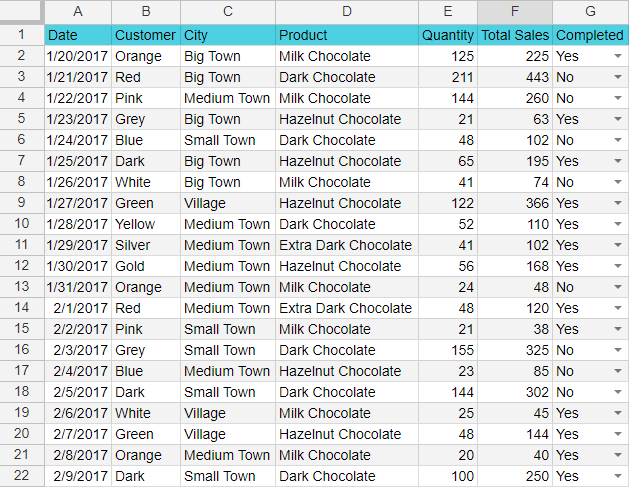
What can be interesting for us to see here? First, we can highlight those orders that exceed $200 in total sales. We have these records in column F, so we'll use our mouse to select the range of values with the order amount: F2:F22.
Then find the Format menu item and click on Conditional formatting.
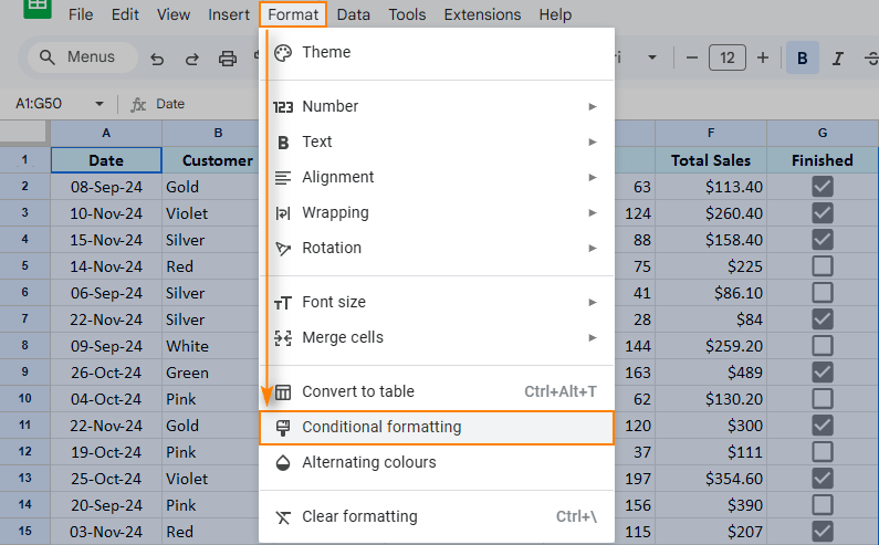
To begin with, let's consider Google Sheets conditional formatting using a single color.
Click Format cells if..., select the option "Greater than or equal to" in the drop-down list that you see, and enter "200" in the field below. This means that within the range we selected, all cells with values that are greater than or equal to 200 will be highlighted using the format we set right at the same place: bold red font in the yellow background.
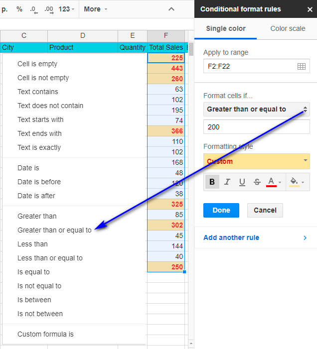
We can see our formatting rule applied right away: all the necessary cells changed their appearance.
You have the choice of setting up conditional formatting not only with one hue but using a color scale. To do this, select Color scale in the conditional format rules sidebar and use ready sets of color. You can also pick hues for the minimum and maximum points, as well as for the midpoint if necessary.
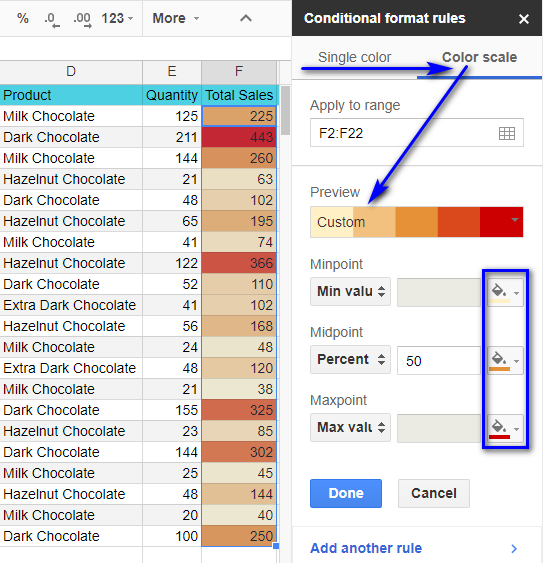
Here we created a color scale where the cells get lighter as the order amount gets smaller, and darker as the sum increases.
Format cells in Google Sheets by multiple conditions
If the color scale seems too bright to you, you can create several conditions under the "Single color" tab and specify a format for each condition separately. To do this, click "Add another rule".
Let's highlight the orders that are over $200 in Total sales, and those that are under $100.
As you can see, we have two formatting conditions here. The first one is for values that are greater than 200, the second one concerns values that are less than 100.

Tip. You can add as many conditional formatting rules in Google Sheets as you need. To delete it, just point to it and click the Remove icon.
Google Sheets conditional formatting with custom formulas
The suggested list of the conditions that we can apply to our data range is quite vast. However, it may still not be enough. Sooner or later you will need to create a condition that can't be described using the standard means.
That's why Google Sheets provide the possibility to enter your own formula as a condition. This formula lets you describe your requirements using standard functions and operators. In other words, the result of the formula must be either "True" or "False".
Use the last item in the drop-down list to enter your formula: "Custom formula is".

Let's see how it works.
Say we want to know which among our orders were made during the weekend. None of the standard conditions works for us.
We will select the range of dates in A2:A22, go to the Format menu and click Conditional formatting. Select the "Custom formula is" item in the "Format cells if" drop-down list and enter the logical formula that will help us identify the day of the week by the date.
=WEEKDAY(A2:A22,2)>5
If the number is greater than 5, then it's Saturday or Sunday. In this case, the formatting we set below will be applied to the cell.

As you can see, all weekends are highlighted with color now.
Here is another example. Let's bring out the orders for dark chocolate with the help of a different format. We follow the same steps to do this: select the data range with the types of chocolate (D2:D22) and use the following condition:
=REGEXMATCH(D2:D22;"Dark")
This function will return "True" if the name of the chocolate type contains the word "Dark".
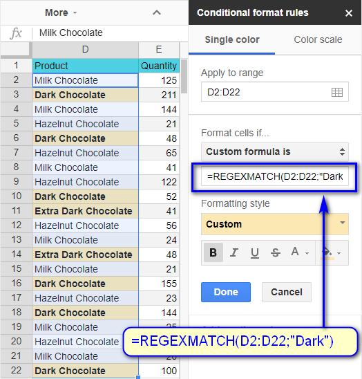
Look what we got: the orders for Dark Chocolate as well as for Extra Dark Chocolate became emphasized. No need to look through hundreds of rows to find them now.
Use wildcard characters with conditional formatting in Google spreadsheets
If we want to format text values, then the standard "Text contains" condition is essential.
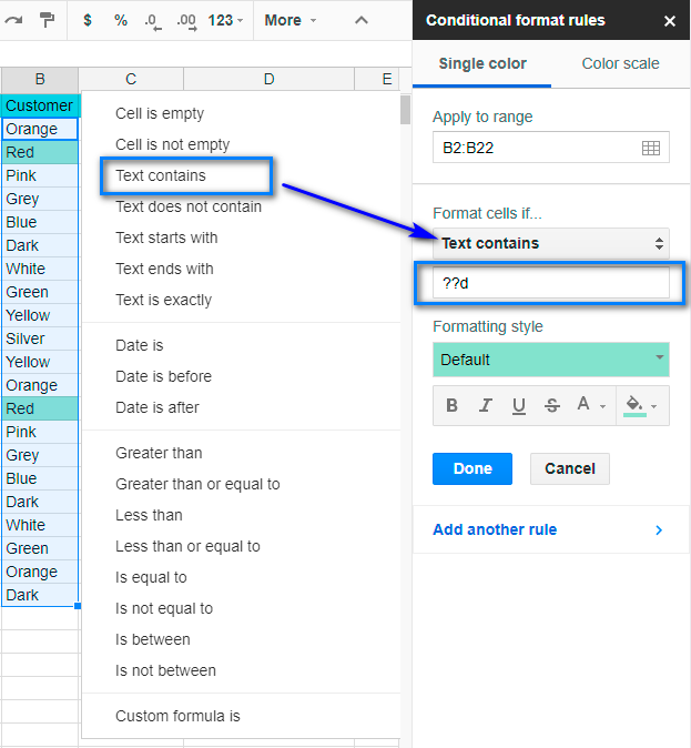
You can use special wildcard characters to add some flexibility to the search condition.
Tip. Wildcard characters can be used in the "Text contains" and "Text does not contain" fields as well as in your custom formulas.
There are two most commonly used characters: the question sign (?) and an asterisk (*).
The question sign corresponds to any single character. For example, as you can see in the screenshot, the text rule that contains "??d" formats cells with such values as "Red", but not such as "Dark".
"??d" means that letter "d" should come third from the beginning of the word.
Use an asterisk to omit zero to any number of characters. For example, a rule that contains "*d*" should format both cells: with "Red" as well as with "Dark" values.
For the question and asterisk characters not to be perceived as wildcard characters in your text values, a tilde (~) is usually added before them. E.g. the text rule that contains "Re?" in our example formats the cells with "Red", while the rule with "Re~?" won't find any cells as it will be looking for the value "Re?".
How to use Google Sheets conditional formatting to highlight entire rows
In the examples we described above, we applied conditional formatting to certain cells of a column. Perhaps you thought: "It would be so nice if we could apply this to the whole table!". And you can!
Let's try to highlight any unfulfilled orders with a special color. To do this, we need to use the formatting condition for the data in column G where we specified if the order was completed, and we shall format the entire table.

Note. Please note that we applied formatting to the entire table A1:G22.
Then we used our custom formula where we specified that:
=$G1="No"
Tip. You need to use the dollar sign ($) before the name of the column. This creates an absolute reference to it, so the formula will always refer to this particular column, while the row number can change.
In other words, we ask it to move down within the column starting with the first row and look for all cells with the value "No".
As you can see, not only the cells that we checked for our condition became formatted. Conditional formatting is now applied to entire rows.
So, let's remember 3 basic rules to conditionally format rows in a table:
- The range to be formatted is the entire table
- We use conditional formatting with a custom formula
- We must use the $ character before the column name
Google Sheets conditional formatting based on another cell
We often hear the question "How do we apply conditional formatting and make it easy to change the condition?" This is not difficult at all.
Just use your own formula with a reference to the cell where you specify the necessary condition.
Let's go back to our sample data with the orders for chocolate in Google Sheets. Suppose we are interested in the orders with fewer than 50 and more than 100 items. We'll go ahead and enter these conditions in column H next to our table.

Now we shall create conditional formatting rules for the table of orders.
We set the range to format to "A2:G22" to keep the table header as it is.
Then we follow the steps you know and use our formula.
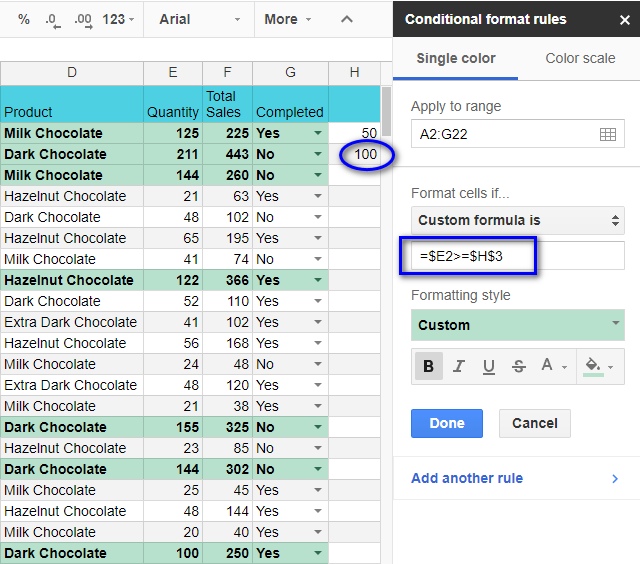
Here is how conditional formatting formula for the orders with over 100 items looks:
=$E2>=$H$3
Note. Please note that you need to use absolute references ($) when using cells outside the table.
A dollar sign before the column name means the absolute reference to the column. If the dollar sign is before the row number, then the absolute reference goes for the row. For more info, please check out this detailed discussion of cell references.
$H$3 in our example means an absolute reference to the cell, i.e. whatever you do with the table, the formula will still refer to this cell.
Note. We need to use an absolute reference to column E and an absolute reference to cell H3 where we have our limit of 100. If we don't do this, the formula won't work!
Now let's add the second condition to highlight the orders with fewer than 50 items. Click "Add another rule" and add another condition just like we did for the first one.
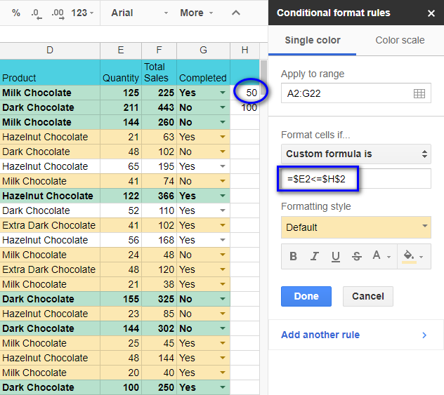
Please see the formula we use in our conditional formatting rule:
=$E2<=$H$2
The largest and the smallest orders are now highlighted with color. The task is accomplished. However, it's not nice that we got extra numbers in our sheet, which may be confusing and ruin the way the table looks.
Placing auxiliary data in a separate sheet would be a better way to go. I will describe it in more detail in my next post when we learn how to create drop-down lists.
Let's switch to sheet 2 and enter these new conditions there.

Now we can create conditional formatting rules for the table of orders by referring to these limits.
Here is where we may face an issue. If we simply use the address of the cell from sheet 2 in the formula, we'll get an error.
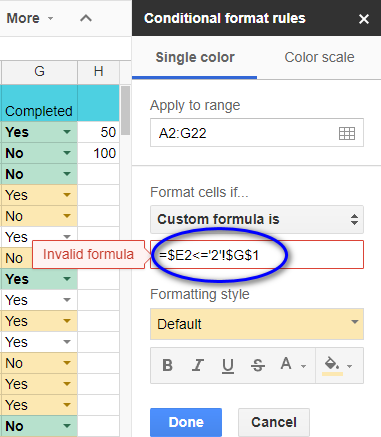
Note. Direct cell references in the formulas for conditional formatting are possible only from the current sheet.
So, what shall we do now? The INDIRECT function will help. It lets you get the cell reference by writing its address as text. Here is how the cell reference within a conditional formatting formula will look like:
=$E2>=INDIRECT("2!G2")
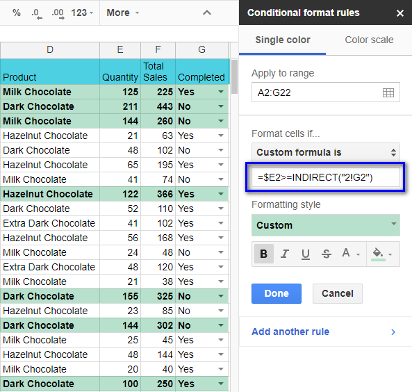
Here is the second formula:
=$E2<=INDIRECT("2!G1")
As a result, we get the same outcome as before, but our sheet is not cluttered with additional records.
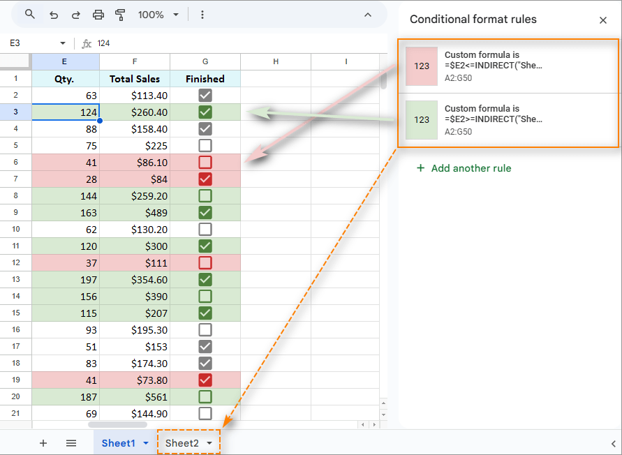
Now we can change formatting conditions without updating the rule settings. It's enough to simply change the records in the cells, and you get a new table.
Google Sheets and conditional formatting based on another cell text
We have learned how to apply conditional formatting rules by using numeric data from a certain cell. What if we want to base our condition on a cell with text? Let's see how we can do this together.
We'll try to find the orders for dark chocolate:
In cell G5 of Sheet 2, we enter our condition: "Dark".
Then we return to Sheet 1 with the table and select the range to format again: A2:G22.
Then we select Format menu, pick Conditional formatting, and enter the following formula into the Custom formula is field:
=REGEXMATCH($D2:$D22,INDIRECT("2!$G$5"))
Tip. Remember that you need to enter absolute references to the range you need to check for the word "Dark" (D2:D22).
The function INDIRECT("2!$G$5") enables us to get the value from cell G5 of Sheet2, i.e. the word "Dark".

Thus, we have highlighted the orders that have the word from cell G5 of Sheet 2 as a part of the product name.
We could make it easier, of course. Our formula would look this way:
=REGEXMATCH($D2:$D22,"Dark")
However, in case we wanted to find a different product, we would have to edit the conditional formatting rule. This takes a little longer than simply updating the value in cell G5.
Remove conditional formatting from your Google spreadsheet
You may certainly need to remove all conditional formats from your table.
To do this, first, select the range of cells where you have conditional formatting applied.
You will see all the rules that you created in the sidebar.

Point your mouse to the condition that needs to be deleted and click the "Remove" icon. Conditional formatting will be cleared.
If you don't remember the exact cell range you formatted, or if you want to get rid of formats as quickly as possible, then select the cell range and go to the Format menu - Clear formatting. You can also use the combination of keys Ctrl + \.
Note. Remember that not only conditional formatting, but all other formats used in your table will be cleared in this case.
We hope that applying conditional formatting in Google Sheets will simplify your work and make the results more graphic.
 by
by
156 comments
In my google sheets table, column A contains text and column F contains text and a total of 911 rows.
On each row, how can I highlight the row if the text in Column F is NOT EQUAL to column A?
E.g.
Cell A6 = "Hello" & Cell F6 = "Hello" then highlight row.
Cell A7 = "Hello" & Cell F7 = "Hi" then do not highlight.
and so on...
Hello!
Apply a conditional formatting rule to lines 1: 911 using the formula
=$A1<>$C1
I hope it’ll be helpful.
Apologies for combining the two, it's Google Sheets.
Thank you for replying.
If the issue still persists, please try clearing cache and cookies in your browser. If this doesn't help, please specify what menu items you follow exactly and where you're being redirected exactly. We'll see if there's anything we can advise you.
When using Excel Sheets on my tablet, clicking on 'conditional formatting' takes me to my files every time.
Any idea why that is and what the solution might be?
Hello,
I'm sorry, do you work with Excel Online or Google Sheets?
Hi Natalia
Thank you for your post as it is very helpful!
I use excel quite often and when I upload the spreadsheet to google drive, the formulas do not always work even though they work prior to uploading the spreadsheet to google drive.
I have 2 questions:
1st question, what is the conditional formatting formula to identify the 2nd lowest value in a column?
2nd question is a little more complicated. I have a spreadsheet which includes 2 columns, one of the columns consists of banks I work with, and the 2nd column is the interest rate they are offering. Sometimes more than one bank is offering the same interest rate.
On the same spreadsheet, I want to set it up so that when I enter an interest rate in a separate cell on this same spreadsheet, the bank or banks that are offering this same rate will automatically populate.
The formula below works before I upload the spreadsheet to google sheets, but doesn't work once the spreadsheet is uploaded to google drive.
=IF(ROWS($C$17:E20)<=$C$16,INDEX($K$2:$K$33,AGGREGATE(15,3,($L$2:$L$33=$D$16)/($L$2:$L$33=$D$16)*(ROW($L$2:$L$33)-ROW(P$1)),ROWS($C$17:E20))),"")
Thank you!
Hi Jimmy,
Thank you for your feedback.
Note. We keep that Google account for file sharing only and don't monitor its Inbox. Please do not email there. Once you share the file, just confirm by replying here. We'll look into your task and try our best to help.
Hi, great article, very helpful, thank you.
I have a question. Well, a two-part question. Is it possible to set conditioning in a way that people will not be able to see the conditioning? For example, if I want to set questions that people answer, and if the answer is correct, it's one colour, and if the answer is incorrect, it's a different colour? I can do the colour thing, no problem. However, users are also able to see the formatting, so they would be able to see what the correct answer is just by checking the conditions of the formatting. Is there a way around this?
If there isn't. then is there a way to link the formatting to a separate sheet?
Thanks,
Mike
Hi Mike,
I'm sorry, I'm afraid it's impossible to link the conditional formatting to a separate document.
However, you can create the sheet with the correct answers, protect it from editing (so only you could edit it), and then hide the sheet. People without the permissions won't be able to unhide it.
You can also hide rows or columns with the answers. People without the permissions won't be able to unhide them as well.
Thanks, but I have also tried that too - I have one doc, with questions and spaces for answers on the first sheet, and a second sheet serving as a control sheet.
But now I don't know how to set the conditional formatting so that when the answer entered on to sheet 1 matches the answer on sheet 2 the answer shows in blue, and all other answers show in red.
Currently, all answers show in blue, regardless of what I try. So I'm doing something wrong :-)
Thank you for replying, Mark.
Sorry, it's hard to tell what you're may be doing wrong without seeing the data and the rules. For me to be able to help you better, please consider sharing an editable copy of your spreadsheet with us (support@apps4gs.com). You can replace any important information with some irrelevant data, just keep the format.
Note. We keep that Google account for file sharing only and don't monitor its Inbox. Please do not email there. Once you share the file, just confirm by replying here.
Is it possible to shade the text of a cell if it's a formula? So if the cell contains a formula, it's output will be blue?
It doesn't need to be a specific formula, just for any cell that contains a formula, change it's color.
Sure,
assuming you want to check and colour cells in A2:A10, apply the conditional formatting to this range with a Custom formula as a rule and a formula like this:
=ISFORMULA(A2:A10)
Working on a Baseball League Google Sheet. Worksheet MPL contains all of the player data then there are individual Team Worksheets. Every player has a unique Numerical player code and this code is on every team sheet and on the MPL. The MPL has a column called (TYPE) that contains either nothing or an alpha value (UNC, UNL or MUP). There is no TYPE column on the Team Worksheets.
What I am trying to do is create a Conditional Format on the Team page that will respond to a Formula IF/AND query by formatting THE selected area specific colour.
Here is the formula I am using:
AND($G$8:$G$62=INDIRECT("Master Player List!$Z$1:$Z$1521"),INDIRECT("Master Player List!$C$1:$C$1521")="UNC")
Column Z on the MPL contains a unique number for every MLB Player
Column C is either blank or contains one of the following values UNC UNL or MUP
Column G on the target worksheet contains the same unique number for every MLB Player
Thanks for any help you can provide.
John
Hello John,
For us to be able to help you, please share a small sample spreadsheet with us (support@4-bits.com) with your source data and the result you expect to get. I kindly ask you to shorten the tables to 10-20 rows. If you have confidential information there, you can replace it with some irrelevant data, just keep the format.
Note. We keep that email for file sharing only and don't monitor its Inbox. Please do not email there. Once you share the file, just confirm by replying here.
Just sent the shared file to your site.
Thank you John,
We've got the file. One of our tech guys figured the easiest way would be to pull Col3 to each individual team sheet with your Query as well. Once you mention it in the formula, the column with types will appear as the last one – Q. Then, use formulas like this in your conditional formatting:
=$Q:$Q ="MUP"
If you don't need columns with types in those team sheets, you can hide them – the conditional formula rules will still work.
Thank you for your help. I was trying to find a way to do it without having to add 30 more columns to the Workbook. I have other similar cross sheet formulas that I am looking at but may have to just forget about it then.
I got the Answer..
Apply to range: B1:C
Format cells if... Custom Formula is...
Formula: =IF($A1<>"",B1="")
Format:
It may be helpful to someone..
Thank for your comments Rishabh.
Unfortunately, your solution doesn't work correctly.
I'd suggest creating 2 different rules in the following order:
I have a problem..
For example:
3 COLUMNS: A, B, C
Column C and Column B is to be highlighted if column A is filled.
Once C is also filled, the highlight on cell in column C goes away.
Once B is also filled, the highlight on cell in column B goes away.
Could you please help me with a condition for this..
please let me know what to do..
Hi there. Thank you for this great article.
My question is this:
I have two columns, A and B. Column A is my Due date and column B is my Shipped Date. All of column A has already four conditional formatting applied as follows:
Condition 1: Format cells if greater than =today()+7 - background green
Condition 2: Format cells if is between =today()+1 & =today()+6 - background yellow
Condition 3: Format cells if is between =today()+0 & =today()-14 - background orange
Condition 4: Format cells if less than =today()-14 - background red
Now I would like to strikethrough the text in any cell in column if there is a value in the corresponding cell in column B. How do I format that? Please help?
Thank you!
Hi Jon,
Formatting styles let you not only change the background color of cells but also alter the font in different ways. Simply create a new rule (for example, =B1:B10<>""), apply it to A1:A10, and choose Strikethrough in the Formatting style of the rule.
Thank you very much.
My question is how can I conditionally format a ROW of cells for 1) a color based on a value of one cell AND 2) have it do a color scale based on the value of another cell. Example: I have the follow row
Species Quantity Endangered Severity Organization
If I want to create a chart that will color all rows pink if the organization is "alpha," all rows blue if the organization is "beta," all rows green if the organization is "Charlie," but have it be a lighter pink, blue or green if the severity is 1, and a darker color if the severity is 5. How can I put that formula in?
Thank you!
Hello Lara,
I'm afraid you won't be able to put all these conditions into one formula for a single rule.
For me to be able to help you out, please share a small sample spreadsheet with us (support@4-bits.com) with 2 sheets: your source data and the result you expect to get. I kindly ask you to shorten the tables to 10-20 rows. Once you share the file, just confirm by replying here.
Thank you.
Excellent article team.
The variation I am looking for is how do I highlight more than one text item; i.e. if my range includes ANY of "red", "white" or "blue", I want to highlight (at least the cell, maybe the row).
(Would your suggestion be case-insensitive?)
Would your response also work for filtering?
Thank you for the feedback, Colin!
You can create three separate rules for when Text contains: red / white / blue (case-insensitive).
Or use three custom formulas like this to color entire rows (case-sensitive):
=REGEXMATCH($B1:$B10,"white")
In this case, you apply the rule to the entire table but use only the column where words appear in the rule. This case is described here.
The rules work only for visible cells.
Hello there. Is it possible to have 1 rule "handling" the color of the text and 1 rule handling the fill color of the cell?
For example, I have in the range A2:Z300, a rule (=$B2="Something") that determines the fill color of the entire row.
Then I have another rule (=A2="somethingElse"), again in the same range that determines the text color of the cell that contains "somethingElse". To me it seems that the rules are working the same way it works when you have the "stop if true" enabled in excel. Is there a way to disable this?
Ty.
Hello Dimitris,
As for your first rule, make sure it is applied to the entire range with your data. Then all rows where B is "Something" should be coloured.
As for the second rule, try picking Text is exactly instead of Custom formula and enter ="somethingElse". Again, make sure to apply it to the entire range. Then all cells with "somethingElse" will change the font colour.
If you're still having difficulties, please share your file with us (support@4-bits.com) with your source data and the result you expect to get. I kindly ask you to shorten the table to 10-20 rows.
Then confirm sharing by replying here and I'll look into it.
Good day
How can i highlight a entire row as soon as col A has text in it instead of a number
Good day,
Please try this formula in your conditional formatting:
=COUNTIF(A1,"*")
Make sure to apply the rule to the entire table.
Is it possible to exclude $0 value in colour scale? e.g. e7:p48 contain monthly spends per client, where client has not started spending or does not spend value comes in as zero. I need the colour scale to show lowest monthly spend and highest, excluding zero value - is this possible?
Hi Lara,
the combination of MIN and IF lets you find the lowest value excluding zeros:
=ARRAYFORMULA(MIN(IF($E$7:$P$48<>0,$E$7:$P$48)))
for the highest excluding zero, try this one:
=ARRAYFORMULA(MAX(IF($B$1:$B$9<>0,$B$1:$B$9)))
HI,
I'm trying to create a search box that will allow users to enter a name and the items that start with the same first letter will be highlighted and all brought to the top of the sheet or open in a new window.
Hi Mary,
If the standard filter doesn't work as you need, I think you can make use of the QUERY function. You can learn a bit more about it on this help page.
Or have a look at our Advanced Find and Replace add-on instead ;)
Hi,
I am currently doing a column-date based formatting in which when a certain task is done passed the deadline, it will highlight the cell red and green if it is done before or exact date of the deadline.
Example:
Cell F11(Deadline) = June 30
Cell G11(Date Done) = July 1(Passed deadline)
and what I want is for G11 to highlight in red or green(depends on the date) accordingly to the value if F11 without changing the value within the formula on the conditional format rules as to we have different values for the deadline.
Thanks in advance.
Hi Roque,
If I get your task clear, you need to create two conditional formatting rules:
1) To color cells with green:
=AND(ISBLANK($G11)=false,G11<=F11)
2) To color cells with red:
=G11>F11
Make sure to apply the rules to the range with your table.
Thanks Natalia. It worked!
Yay! Good to know, Roque. :)
HELLO,
I am trying to format a column base on the date of the case is less than today + 7 weeks.
do you have a solution.
Thank you.
Hello Idir,
For us to be able to help you better, please share a small sample spreadsheet with us (support@4-bits.com) with your source data and the result you expect to get. I kindly ask you to shorten the table to 10-20 rows.
Note. We keep that email for file sharing only and don't monitor its Inbox. Once you share the file, just confirm by replying here.
Thank you.
Hi Natalia!
I need your help!
I below is a small illustration of my table. the 1st row "1 2 3 4" runs till 31 and represents the days of the month. So my objective is to highlight entire column based on the current day of the month, and also highlight the name of the person where their value is "1" on current day of month
1 2 3 4
TOM 1 0 1 0
JACK 0 1 1 0
JILL 0 0 0 0
=$1:$1=DAY(NOW())
This works for highlighting the column based on day of month, but I cant get the formula to high the name base on the value in the current day.
What I have so far:
=INDIRECT(CHAR(DAY(NOW())+64)&":"&CHAR(DAY(NOW())+64))=1
Thank you so much!
Hi Amos,
What if you try the following?
=AND(2:2=1,$1:$1=DAY(NOW()))
This highlights all cells with "1" based on the day of the month (today).
Hi Natalia,
Thank you so much for your reply. I managed to solve it in a different way.
I created an extra column (hidden) with the formula =HLOOKUP(DAY(TODAY()),/*my data range*/,6). Then in my 1st column where I have the names, my custom formula for the conditional formatting was to check and highlight the name if that hidden column contains a '1' in that row. But thanks a lot anyways :)
Hi Amos,
It's good to know you found a solution that works for you!
Thank you for sharing your workaround with us. :)
I've shared a sample sheet as I cannot get it to compare
Just to confirm, I'd like to highlight any entries in column H that apear on sheet IP in column A
Thank you for the file, Daniel.
I wasn't able to make the formula work on your data though it perfectly runs on mine.
However, I've come up with another formula for you to try in conditional formatting:
=AND($H3<>"",MATCH($H3,INDIRECT("IPList!A:A"),0))
Please let me know if it works.
Thanks Natalia, that works perfectly
I am having the same issue as Natalie
I would like to format row H, if the value matches any cell from sheet IP in row A
This is what I have, but it does not seem to work
=$H3=INDIRECT("IP!A3:A")
If I compare to only 1 cell from sheet IP then all is well
=$H3=INDIRECT("IP!$A$3")
Is this possible?
The formula like you wrote does work for me. I even mention this way in this article.
Please make sure you apply the rule to the correct range, for example, H2:H20.
If this doesn't work, please share a small sample spreadsheet with us (support@4-bits.com) with your source data and the rules you use. I kindly ask you to shorten the tables to 10-20 rows.
Note. We keep support@4-bits.com for file sharing only and don't monitor its Inbox. Please do not email there. Once you share the file, just confirm in this message thread.
I'll look into your task and do my best to help.
Hi,
I would like to ask 1 question. when doing a conditional formating,
for the format rules, can i use text that contains "a range"
for example, my data range is D2:D50, and i want to highlight cells that has duplicates/ names that are found in range D60:D70.
Is that possible??? have been trying to solve this for 2 days
thank you so much...
Hi Natalie,
Since you have two ranges that you'd like to compare for duplicates and highlight, please read this article.
I am trying to format an entire row to become a color if a particular cell is not empty. My research indicates that the formula that is supposed to work for this is =$H4034" ", (4034 is the row I'm in at the moment) but it isn't working, possibly because there is already another formula (for how a date needs to look) for the whole spreadsheet...? Because of this, I've tried any number of formulas based on how a date looks when entered, using numbers, using the "/" symbol, using "?" & "*", and I can't get any of them to work. Please help. I've been trying to figure this out for a week, and I'm at my wits end.
Alex,
you should be able to color entire rows where H contains data with this formula for conditional formatting:
=$H1<>""
Make sure to apply the rule to your entire table, for example, $A1:$H5000.
I would like to be able to colour a whole row based on a date in one cell. I want the row highlighted if the date in one of the cells is before 3 years ago today.
Thanks.
Suppose your table is in A2:J11, with dates in column J. Here's the formula for your conditional formatting rule:
=DATEDIF($J2,NOW(),"y")=3
Pick the color to highlight rows and apply the rule to the range &A2:&J11.
Do you know of a way to make a list from formatted cells? I am trying to create a new list from highlighted cells in a column.
Hi JD,
Unfortunately, you won't be able to do that with the standard Google Sheets features. You need to create a script or look for a special add-on. But I'm afraid we don't have a tool for this task.
Hello,
I am trying to organize a table of data with cells that contain both numbers and words. Each cell has datum similar to: "25.5 Minutes". I would like to highlight all cells that have more than 120 Minutes, but cant seem to find a way. Any help would be most appreciated!
Hello Dillon,
Assuming your values are in column A, use the following formula in the Conditional formatting rule:
=(LEFT(A1:A3,FIND(" ",A1:A3)-1)*1)>=120
Excellent article !!
I got lost about "$3" of the "=$E2>=$H$3" I understand the "if E2>= H" but what the "$3" means? Why not simply "=$E2>=$H2"?
We compare all cells in column H with one and the same cell - H3. The dollar sign makes sure of that: it doesn't allow the reference to change the number to H4, for example, when comparing with E4.
You can read more about types of cell references here.
I need to find and remove duplicates from my google sheet. The formula provided does not seem to work. The instructions are confusing. I wish someone could explain it to me like I was a 12-year-old. Very frustrating. =countif(A:A,A1)>1. I need it for column C so =countif(A:A,C1)>1?
Hi Rob,
What formula did you use? If I'm correct, none of them is for finding duplicates in this article.
Your first formula will check if a value from A1 appears in column A. Your second formula will scan column A for the record from C1.
Perhaps, this article will answer your question in a way. If not, feel free to check the tutorial for Excel. Most of the formulas will work for Google Sheets as well.
How do I format a cell to change colour if it is still empty after a certain day.
For example I want it to turn red 28days after 07/01/2019 if the cell is still empty.
Supposing a cell to change the color is A2. Try this formula in your conditional formatting:
=AND(ISBLANK(A2),(TODAY()>(DATE(2019,7,1)+28)))
Hi,
I have a gantt chart and I'm trying to show coverage in main headers for the gantt chart when there is a different color cell. So for example,
row D5:BD7 and I want to highlight row 5 when there is a colored cell in rows 6 and 7. So let's assume that row 5 will be orange, and there is orange colored in G6:P6, AM6:AQ6 and there is orange colored I7:M7, R7:Y7, AG7:BC7.
How do I put in conditional formatting to make this happen in row 5?
Thanks!
Hi,
I'm sorry, I don't believe it's possible with standard Google Sheets tools. This would require formulas to identify colors in cells.
I think you'll need to use scripts to solve this task.
Okay I have a weird thing going on: Anytime I type the word "Lenten" or "Lent" in a cell, it turns green. There are no conditional formatting active on the entire spreadsheet. Any ideas?
You're searching for "lent", so when you type it into a cell it is showing up green because it's highlighting the search term. Everyone does this at some point. Some of us do it more than once. :)
Hi,
Thanks for the great help to various questions. I have created a simple "To do" list for my office tasks. As soon as a task row is completed, I have set conditional formatting to strike how that task and mark status and percentage in status and progress columns.
This works for the tasks that are of one time like "Defining Scope of the project". However, in case of recurring tasks like "Send the weekly Status reports", what I am looking for is - as soon as one row for the task "Weekly Status Reports" is Striked out as completed, another normal row of the same content is inserted below it (by same content I mean the content which was there before being striked out, the percentage set to blank and status also set to blank) (by normal I mean which is not striked out). I want to do this since this will be a recurring task.
Please can you help me on this?
Dear Sir,
Please Suggest me how i can apply Conditional formatting as per below given data:
A B C D
RE-ORDER LEVEL MIN STOCK LEVEL Max Stock Level NEED COLOR CODING BY
CONDITIONAL FORMATTING FOR
A,B,C
Regards
Trivedi Singh
hi, in excel there is a function that help us to find values replicated, but in drive i cant find this options... help please
Hi, Daniel,
Most of the functions that work in Excel work in Google Sheets as well.
You can try building the formulas described in this blog post to find replicated data in your spreadsheet.
Alternatively, we have a special add-on designed to look for duplicate and unique values in Google Sheets. It's called Remove Duplicates. You can evaluate the tool for 30 days for free and see if it works for you.
Hope you'll find these tips useful.
Is it possible yet to highlight just text within a cell, not the whole cell in Google sheets?
Thank you for your question, Patricia.
Conditional formatting in Google Sheets lets you change not only the background color of cells but also font color.
When you set the rule, simply pick the color you need using the Text color tool (the icon with "A") and make sure the Fill color is set to None.
Hope this helps.
need help please with following
column A Column B Column C
1 Monday Site 1 employee 1
2 Monday Site 2 employee 2
3 Monday Site 3 employee 2
4 Tuesday Site 1 employee 1
5 Tuesday Site 2 employee 2
6 Tuesday Site 3 employee 3
7 Wednesday Site 1 employee 3
8 Wednesday Site 2 employee 1
9 Wednesday Site 3 employee 2
how do i make c3 change colour in google sheets because it matches as employee cant be assigned to two sites in one day
Hi,
Great post. Any chance when you do your formatting to sort the value by colors. In other word get for exemple all your green values at the top and the rest following.. thanks a lot!
Hello! Hoping you can help.
I am trying to organize a large event (reunion). I have everyone's name typed in to a spreadsheet and a google form linking to their responses of coming or not coming. As they fill out this form, is there a way to have their name turn green on the master list of names, so that I can easily see who has not answered the google form? Rather than having to go through each name and manually check it off the master list? Thanks!
Can you use "AND" statements in Custom Formulas for conditional formatting.
I am trying to conditional format based on two conditions, e.g.
If (A2 = "text") AND (B2>indirect("sheet1!A2))
I tried the following:
=AND(F2="Lower", E2>Indirect("Summary!H$2)) But seems to give an error?
Any thoughts would be greatly appreciated.
Thanks
Hello, Damien,
AND can be used in conditional formatting, and the formula you use looks fine.
I kindly ask you to share your sample spreadsheet with us (gapps.ablebits@gmail.com) where your custom formula doesn't work.
We'll look into the file and do our best to advice you.
Hey,
Currently, I am using conditional formatting to color a cell based on the number from a different cell. I need to do a total of 4 colors for 4 set of range so I am using custom conditional formatting for each range. For some reason, only 3 of my 4 conditions are working. how can I fix this problem and also, is there a simpler way of doing such a format?
I was able to do a conditional formatting for an entire row by doing =$E1="Speech" however this is only highlighting rows where the cell equals "speech" and I would like to do it for all that CONTAIN "speech" is this possible?
Hello, Joanna,
Please try to use the following formula in the Custom Formula field instead of the one you mentioned:
=COUNTIF($E1,"*speech*")>0
Hope this helps!
How to apply conditional formatting in colums for duplicate text with different color (same as color scale, but for text)
I have a code that timestamps when i make a change to a cell, i now want to doa conditional format that an hour after that timestamp it turns red so it stands out for me to follow up.
also when i am creating conditional formats when i delete a row it mess's up which cells it does on "apply to range"
Hello,
I have a list of student in columns B and C (last name in B, first name in C).
I have checkboxes in column A. I want the students names to turn red when the checkbox is not checked (ie, it has a value of "FALSE).
I have set the range in the conditional formatting as B3:C58, becuase that's where the list is, then I select "text contains", and type =A3:A="FALSE".
However, nothing is happening when I do this, even though there are many unchecked (ie, "FALSE) checkboxes in column A.
Please advise!
Menachem:
Are each of the checkboxes linked to another cell?
If not, link the cells to another cell and format that cell based on it's True or False condition. If that works, you should be able to change the color of the cells containing the names based on the value of the cells that contain True or False.
Hi,
I am trying to create a traffic light system that transfers a Green from master page 1 to Green on page 2 and 3.
I am using formula =IF("Page 1!D5"="Green",1,0) and format green works great for single cell.
When I try =IF("Page 1!D5:D10"="Green",1,0) I get no formatting even if all cells are Green. Is there a way to make this work.
I have 3 conditional formats so Amber and Red also
KR
Derek
the section above on INDIRECT has the answer you seek. I do this sort of thing all the time. Try This:
=IF(INDIRECT("'Page 1'!D5:D10")="Green",1,0)
Hi there,
I use conditional formatting on a row (ex. E4:T4) -> I need this format on every single row until E1000:T1000. If I copy and paste special (format only) i get the conditional formatting to cover the range of E4:T1000 insted of:
E4:T4
E5:T5
E6:T6
etc..
E1000:T1000
Is there a short cut to make the conditional formatting for every single row instead?
Hope for help.
BR Martin
How can I create a formula so that the cell that is the greatest, second greatest and third greatest will be highlighted, each in a different color?
For example: my list of numbers is 12, 24, 19, 10, 3, 5, 30. I want it to highlight 30 (the greatest number) in red, 24 (the second greatest) in hot pink, and 19 (the third greatest) in baby pink.
What formula would I use/how would I do that?
Thank you!
Hello,
If I understand your task correctly, you can make use of conditional formatting in Google Sheets described above.
Conditional formatting allows coloring cells depending on the values they contain. However, you will need to use some formulas there to find if the number (use IF function) is the greatest, the 2nd greatest, etc. (MAX and LARGE functions).
Hope this helps!
I am trying to create a formula that will transfer a cell with all formatting saved.. IE: I have a list of names in several cells... all names are different colored, some are lined through and some cells have different background colors.... If I use ='PLAYER'!A1 the name copies over but all formatting is lost.... What formula would I use to carry all formatting to the cell I am coping into??
Hello, Pam,
I'm afraid there's no formula in Google Sheets that would transfer the formatting of one cell to the other one.
The easiest way to copy formatting in Google Sheets is using paint format tool on the Google Sheets toolbar:
https://support.google.com/docs/answer/161768?co=GENIE.Platform%3DDesktop&hl=en
Another, though a bit more challenging way would be to create conditional formatting rules (described above) and apply them to your new cells.
I have a question. is there a formula or way, where a cell changes its value when you change the value of the the other. like for example. if on cell contains 5 and the other cell with change to 0 since may desired formula is "put 0 if the value is less than or equal to 5 if not put 5"?
thanks
Hello,
yes, there is a function that is designed just for cases like this, it's called IF. Please take a look at this article of ours about it:
https://www.ablebits.com/office-addins-blog/if-function-google-sheets/
Hi, Alexander! Your description is excellent (clear&detailed). Thanks.
I have only one question which is not covered above. How can I refer to a named range (i. e. cell or range)? It doesn't work for me.
Thanks in advance for your response.
Best regards, Gábor (Budapest, Hungary)
Hello,
I'm afraid it's impossible to use named ranges directly in conditional formatting. You need to use INDIRECT function with the named range in double quotes.
Hope this helps!