Google Sheets lets you manage rows in many different ways: move, hide and unhide, change their height, and merge multiple rows into one. Special styling tools will also make your table easy visually appealing, easy to understand and work with.
Quick ways to format Google Sheets header row
Headers are an essential part of any table – it's where name the whole content. That is why the first row (or even a few lines) of your table in Google Sheets is usually turned into a header row where each cell hints about what you will find in the column below.
To distinguish this row from others right away, you may want to change its font, borders, or a background color. The following tools will help you format Google Sheets header row:
- Format option in the Google Sheets menu.

- Standard formatting tools on the Google Sheets toolbar.

- Table Styles add-on for Google Sheets.
Table Styles helps quickly format tables in Google Sheets (and header rows specifically). After you install it, you'll find it under Extensions > Table Styles > Start:
Mainly, the styles differ in their color schemes. However, you can format different parts of the table in different ways, whether it's a Google Sheets header row, left or right column, or other parts. This way you will personalize your tables and highlight the most important data.

The main advantage of Table Styles is its ability to create reusable styling templates. Just click on the rectangle with a plus icon (the first in the list of all styles) to start creating your own style. A new template will be created, and you'll be able to adjust it to your liking.
Note. The default styles that exist in the add-on cannot be edited. The tool lets you add, edit, and delete your own styles only.
Choose the part of the table that you want to change, set its appearance, and click Save:

All these options make Table Styles a great extension for Google Sheets that formats entire tables and their separate elements, including Google Sheets header row.
Tip. Learn other ways to format your Google Sheets table from this blog post.
How to color every other row in Google Sheets
Unlike formatting of the header row, there are some tools designed specifically to color every other row in Google Sheets.
1. Use alternating colors
- Select the table where you want to color every other row.
- In the Google Sheets menu, find Format > Alternating colors:

- The corresponding window will appear where you'll be able to double-check the range, choose header/footer if your table has them, and pick the style for your rows:

You can color every other row in Google Sheets using one of the default styles or opt for customizing colors.
2. Use Table Styles add-on
Table Styles add-on is equally good for coloring every other row in Google Sheets. Additionally, you can not just color rows, but set up their text formatting:
- Select the table where you want to color every other row.
- In the Google Sheets menu, go to Extensions > Table Styles > Run:

- Tik the box for Alternating colors (header/footer row as well if needed):

- And tweak all the formatting settings you need to color and format every other row in Google Sheets.
Tip. Save these as your custom style & reapply whenever you need.
How to move rows in Google Sheets
There are 2 ways to rearrange your table & move one or more rows to another place:
- Google Sheets menu. Highlight your line and choose Edit > Move > Row up/down. Repeat the steps to move it further.

- Drag and drop. Select the row and drag-and-drop it to the needed position. This way you can move the row a few columns up and down.
How to hide and unhide rows in a spreadsheet
All tables may contain lines with data used for calculations but unnecessary for displaying. You can easily hide/unhide such rows in Google Sheets without losing the data:
- Right-click the line you'd like to hide.
- Choose Hide row from the context menu:

- Row numbers won't change, but two triangles will prompt that there is a hidden line. Click on those arrows to reveal hidden rows back:

Tip. Want to hide rows based on their contents? This blog post is for you then :)
How to merge rows and cells in Google Sheets
You can not only move, delete, or hide rows in your Google Sheets — you can merge them to make your data look more elegant.
1. Standard Merge Cells
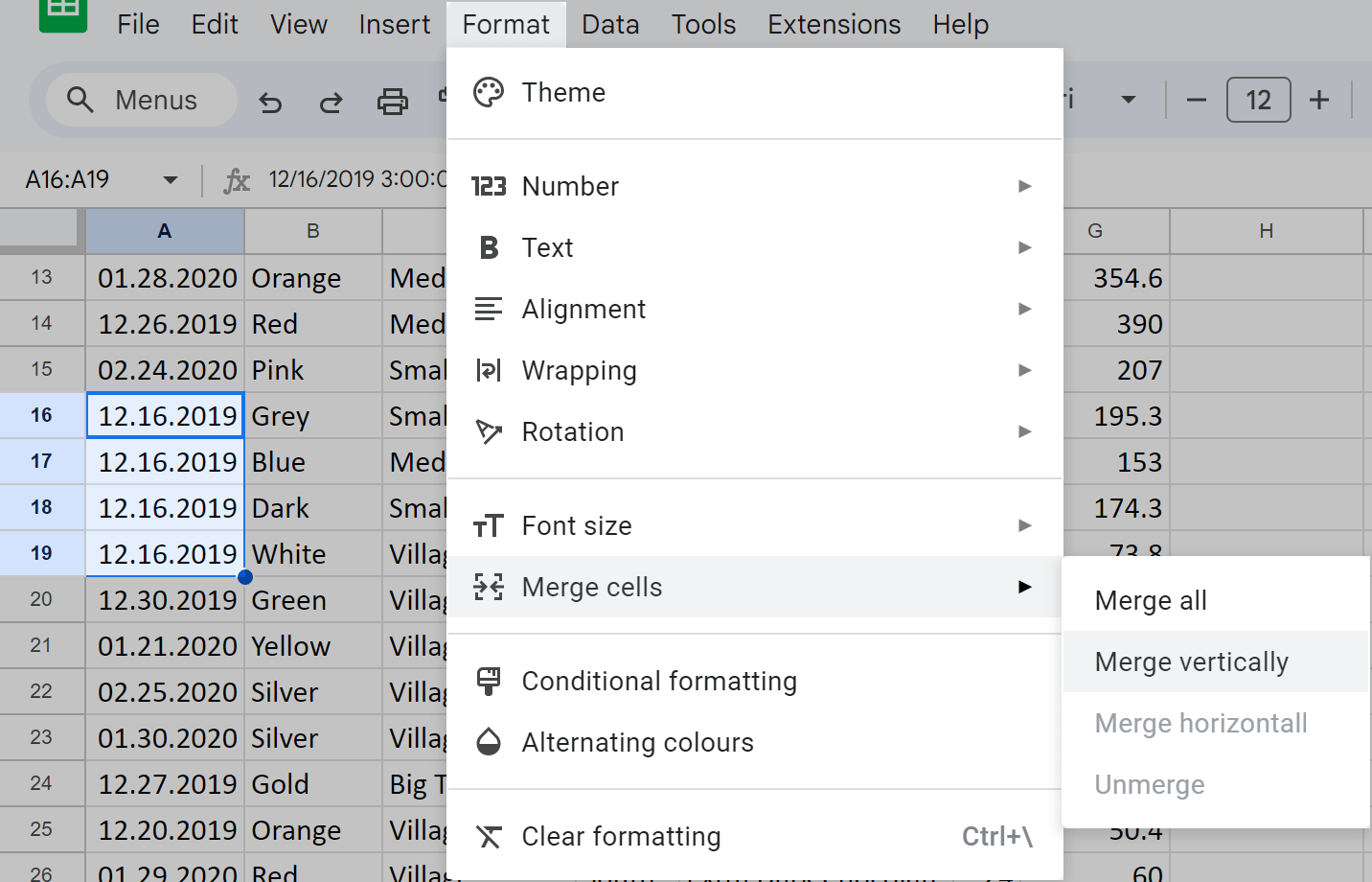
There are a few cells in my table that have the same information (A3:A6) one under another. I highlight them and choose Format > Merge cells > Merge vertically:

4 cells from 4 rows are joined with the data from the top leftmost cell remaining:

2. Merge Values add-on
If the goal is to merge rows in Google Sheets without losing any data, Merge Values tool is a better choice. It doesn't pick any specific value to display — it takes them all and places into one cell. Here's how you use the add-on:
- Install Merge Values to your spreadsheet from the Google Sheets store.
- Run from Extensions > Merge Values > Start:

- Select rows you want to merge.
- Choose to merge values in each column using line breaks as delimiters for instance:

- Click Merge.
Rows in each column will be merged with no data left behind:

The add-on offers a fully-functional 30-day trial period so there's plenty of time to play around & decide whether it's worth buying. These instructions will help you get started.
3. Video: 3 ways to merge cells in Google Sheets
How to change row height in Google Sheets
You can improve the layout of your table by changing the height of some lines, a header row in particular. Here are a couple of easy ways to do that:
- Drag and drop. Hover the cursor over the bottom border of the row, and when the cursor turns into an Up Down Arrow, click and drag the line down (or up) to resize as you need:

- Use context menu. This way is especially useful when you need multiple lines of the same height. Simply select them all, right-click and choose Resize row [N]:

How to count rows with data in Google Sheets
At last, the table is ready, it has all the info, all rows and columns are right where they should be and of the needed size.
But are there any cells that could be unintentionally left empty? Let's count how many lines are actually filled with data.
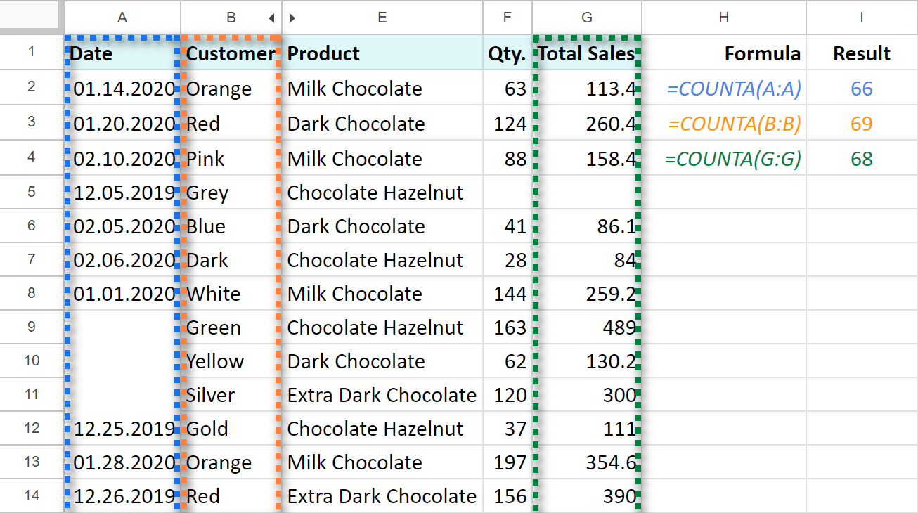
I'll use the COUNTA function: it calculates the number of non-empty cells in the selected range. I want to see how many rows there are with the data in columns A, B, and D:
=COUNTA(A:A)
=COUNTA(B:B)
=COUNTA(G:G)
Tip. To include additional rows that may be added in time to your formula, make sure to use the entire column rather than a definite range as the formula argument.

As you can see, formulas return different results. Why is that?
Column A has vertically merged cells, all rows in column B are filled with data, and only one cell in column C is missing an entry. That is how you can spot empty cells in the rows of your table.
I hope this article will make your work with rows in Google Sheets a bit easier and more pleasant. Feel free to ask questions in the comments section below.
 by
by
11 comments
When your document in Google sheets is very large (18 columns and 50 rows) can columns be hidden behind Column A as you advance across the sheet and also Row 1 in the same manner as you travel down the sheet?
Hello Wendy,
Yes, you can freeze Row 1 and Column A. You will learn how to do it in this article.
dugfreshNClexi was pretty clear. How do you drag a row and have it moved to another place on the sheet AND NOT REPLACE the data. This is very easy in Excel. In Google sheets, I first have to insert a blank row and then drag the old row into that slot. How do I do this in one step like in Excel (as dugfreshNClexi explains, you just hold Shift to do that...)
Hello Jen,
please note that to reorder rows in Google Sheets without overwriting the contents, first you need to click directly on the row number. Not on the blue border of the selected cells, but on the grey row number to the left of the entire row. Please see the first screenshot in this section: the hand marked with '1' shows the exact location where to click.
If this doesn't work for you or you mean something else, please describe in detail what/where you click. Or, even better, make a video recording so I could see what you do exactly.
I want to drag and drop more than one cell at one time.
Eg. How do I drag A1, A5 & A8 and drop them into B10, B11 & B12 all at in one move?
Hello Kimberly,
I'm sorry but drag-and-drop works this way only with rows and columns. If you try to drag and drop cells with data, the contents will simply be copied to the neighbouring cells.
Instead, select multiple cells by keeping Ctrl pressed and then cut their contents with Ctrl+Z. Then select B10 and press Ctrl+V: this will fill B10, B11, and B12 with values from A1, A5, and A8.
dragging and dropping a row _replaces_ the row for me. i have not been able to drag and drop a row _in between_ other rows. in Excel, you hold the shift key down while dragging and you're able to squeeze it in between two rows. what am i missing about the drag & drop functionality in Google sheets?
Hello there,
I'm sorry, it's hard to tell what you may miss since drag'n'drop should work. :(
Please try searching YouTube for instructional videos or refer to Google help page/support:
https://support.google.com/docs/answer/54813?co=GENIE.Platform%3DDesktop&hl=en
I wish I could assist you better.
Great information that solved my issue!
Thanks
Obsolete web page. Move up and Move down have been removed from Google Sheets.
Thank you for the feedback Terry.
Is there a particular task you were trying to find a solution to?
As for the options, they haven't been removed. They are still there, in the Edit menu of Google Sheets (not the context menu in case you were looking there). You just need to select row(s) beforehand to see those options in the menu.