When you use different colors to organize your data in Google Sheets, you might find there are no built-in formulas to easily summarize data based on color. To address this, we introduced several custom functions that take into account both the font and background color of cells for basic operations, making it possible for your Google Sheets to sum by color or count cells by color.
You will find these functions among the smart 40+ features of our Power Tools collection for Google Sheets.
Or get them from this special tool: Function by Color for Google Sheets.
Both offer a 30-day trial period and two subscription plans: 12-month and lifetime.
How to count colored cells in Google Sheets
Let's take one of the most common tasks with colored cells in a spreadsheet: counting cells that have the same formatting. Say, here I have a list of grades and I want to see how many times each test was passed, i.e. count all green cells in a column:
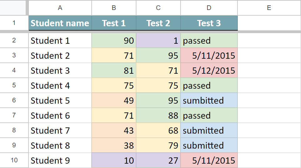
If you're dealing with ranges that include various data types like numbers, text, or dates, consider using the COUNTA function from the Function by Color tool.
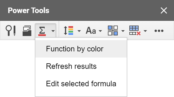
For a start, open the tool to sum by color. In Power Tools, you will see it right on the smart toolbar:
Here are six simple settings you need to specify to get the results:
- The range with the color-coded data that you want to check: I pick the columns with the test results, B2:D18.
- The pattern cell. The function will take its font and/or background color and look for the same in other cells. I pick the fill color of B2 as an example.
- The function. To count cells with a particular number format, it's best to choose the COUNTA function because it is the only one that works with non-numeric values. This way you can be sure that the data format in the cells will not impede the results.
- The place for results. I want my Google Sheets count cells by color in each column so it is three cells for me, B19:D19.
- How to apply it. You can choose to count cells in each row, column, or in all selected cells. As I want to count green cells for each test, I choose to Calculate in each column. If I wanted a general result for all three tests, I'd choose the entire range.
- The formatting of cells with the result. You can have them filled with the same colors as you count by selecting just one checkbox.
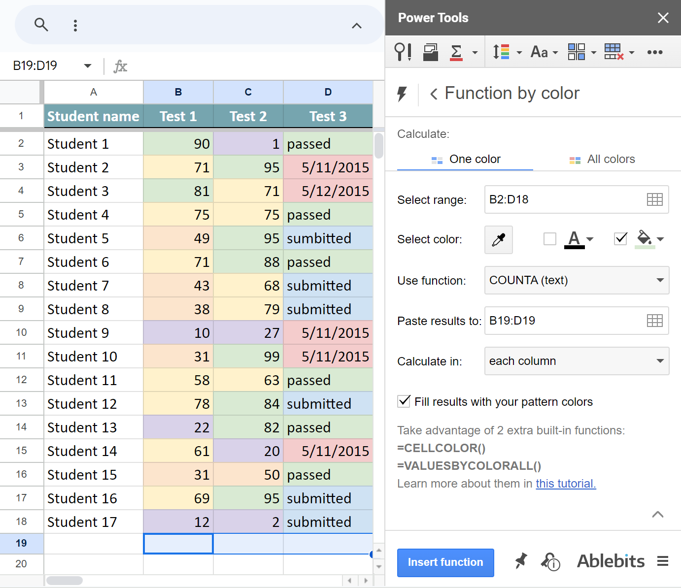
Once I click Insert function, the tool adds the formula under each column, so I will see the results for each test:
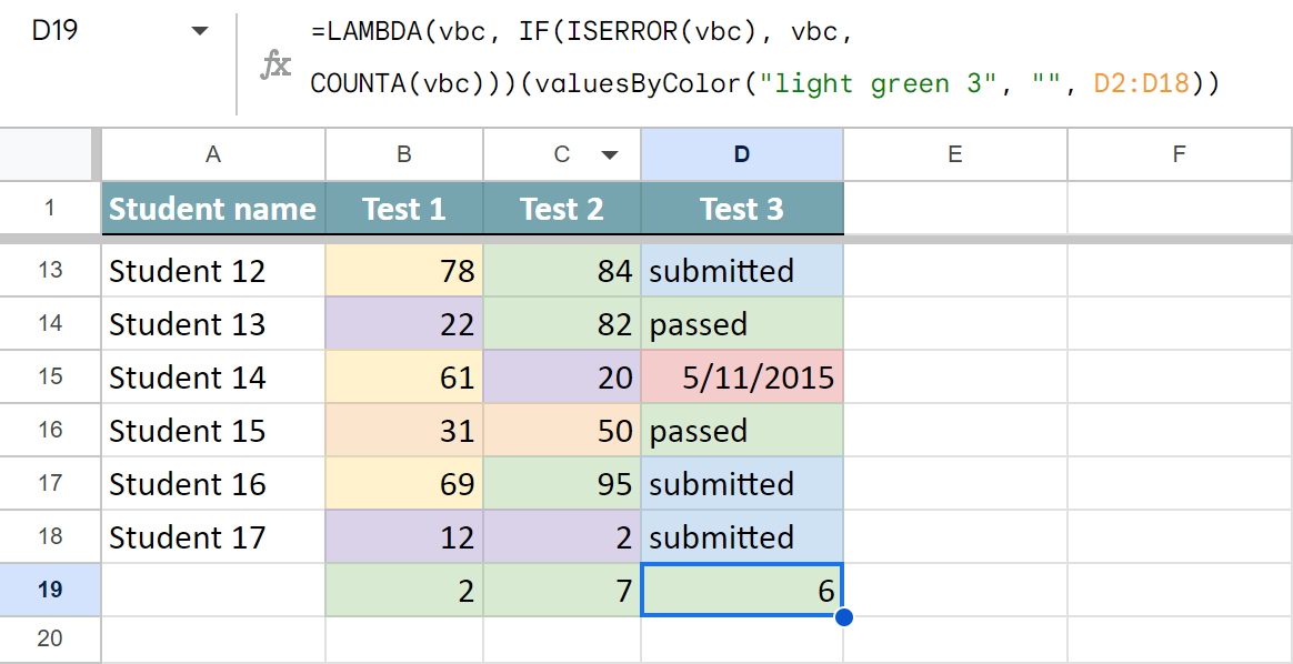
Let me break down its syntax and explain each part:
- =LAMBDA(vbc, IF(ISERROR(vbc), vbc is the service part that enables the formula to return exactly what Google Sheets replies with, whether it's "loading", some error, or the calculation result.
Tip. You'll see this part only for COUNT, COUNTA, and COUNTBLANKS functions because of their peculiarities.
- COUNTA(vbc) is one of standard Google Sheets functions you pick to use with the colored cells. vbc stands for valuesByColor.
- valuesByColor is our custom function that handles colors.
- light green 3 is the cell color considered for the calculations, i.e. the background color of the pattern cell.
- "" is empty since I don't consider the font color of the pattern cell.
- D2:D18 is the range to check for colored cells. In my example, it looks at cells in column B, C & D respectively.
How to sum colored cells in Google Sheets
Say, I'm keeping track of classroom equipment orders. I denote the ordered things by yellow background color, items on the way by blue, and delivered equipment by green:
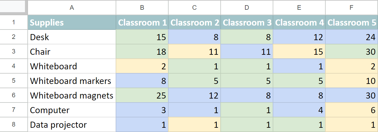
My task is to see how many desks, computers, and other supplies are on the way at the moment. Color is the only difference these numbers have in my table. So I open the tool to sum by color and use the following settings:
- I select the entire range with my data to check it, B2:F8
- I pick C2 as a pattern cell to specify the format of items I want to calculate.
- Select the SUM function to tally numbers from blue cells.
- Pick cells to place the resulting calculations for each item, G2:G8
- To see the number of shipped items for every product, apply the function to each row.
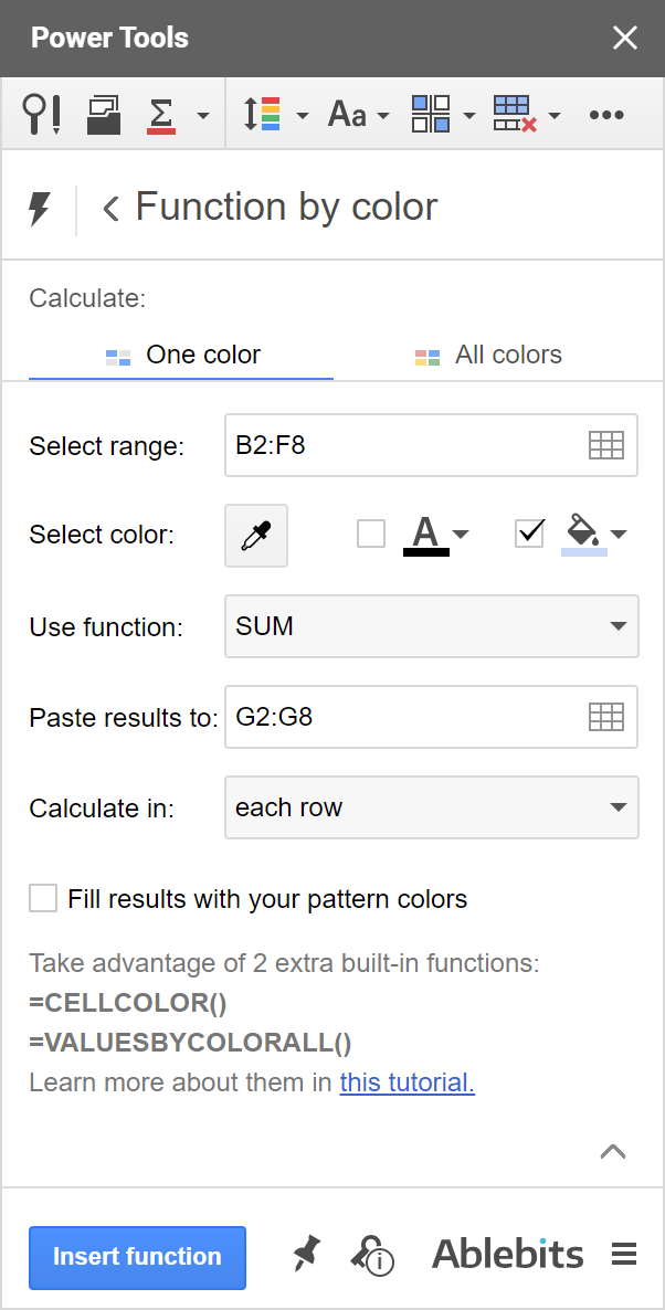
Click Insert function to get the formula after each line in your table.
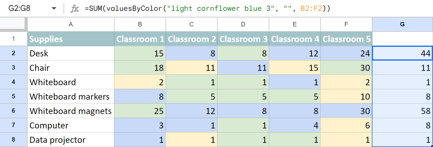
The convenience of getting the formula is that you can modify any of its parts and paste it wherever you need in your Google spreadsheets.
Google Sheets: sum by all colors in the table
The updated Function by Color lets you calculate not just one color per formula but all colors simultaneously.
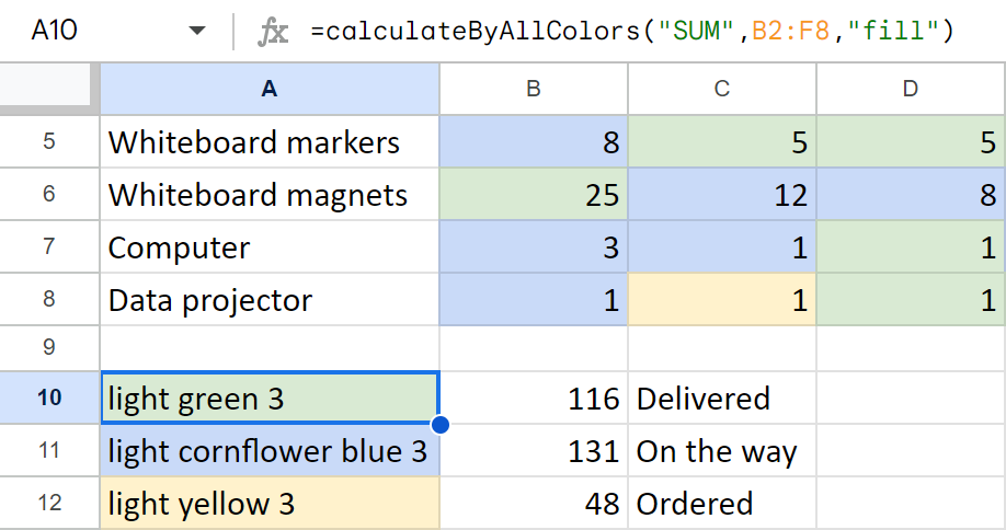
Using the same data as above, I can find the total of all delivered supplies (green), tally those on their way (blue) or those ready for ordering (yellow).
I just need to switch to the All colors tab in the add-on and adjust the same settings:
- The range is the same table, B2:F8.
- I will sum data by all fill colors.
- I also choose to calculate the entire range and have 1 formula inserted in A10.
Note. The formula returns the result in 2 columns: color & the total. So make sure there's enough space to insert the function. The result will show once there's room for it, but until then you may see the #REF! error if other data is on the way.
Update the results
So, Google Sheets doesn't have native functions that work with color. This means your spreadsheet doesn't treat changes to cell formatting as a reason to re-calculate your formula results. The good news is that both workarounds in-store are elementary :)
- You can change any value within the calculated range. Say, you are counting green cells in A1:C254. You can simply add a character to any of the cells in this range, and then remove it to get the updated results.
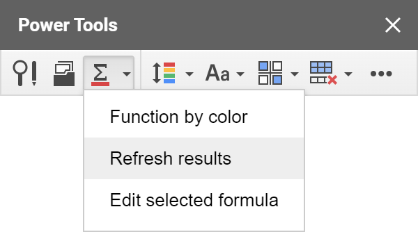
- If you have a lot of valuesByColor formulas in your sheet, click on the Refresh results option (right under the Function by color in Power Tools or under the Extensions menu for the single add-on) to update all formulas in one go.
Edit formulas
Another way to change the result is to edit the entire formula. But if there are only a couple of settings you'd like to choose, you don't have to build the entire formula anew. It is enough to click a cell that already contains a formula and pick the option to edit it:
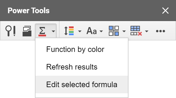
The add-on will open with all the settings necessary to create this selected custom formula. You can adjust some or all of them — ranges, colors, pattern cell, function — and insert everything back.
Troubleshooting
If you see an error in place of the formula, you may be working with a file that has no locale. When this happens, our function doesn't know what delimiters it should use, so it ends up giving you an error. If you see this, please go to File > Settings in Google Sheets and make sure you have the locale set.
Video: How to count colored cells in Google Sheets
 by
by
152 comments
Thanks for sharing this power tool. its very useful for me.
I'm using this tool to sum the amount for numbers in font red, once i change the word to black, the output figure doesn't change on its own, i will have to open the tool to click on refresh result.
is there any shortcuts or auto refresh every time there's changes in the cell?
Hello lin,
I covered this problem and solutions in this part of the article: Update the results
If it's not too much trouble for you, we would appreciate it if you rate Function by Color and maybe write a few words on Google Workspace Marketplace. Your positive feedback motivates us to provide the best experience for you and helps others understand how our product makes their life easier :)
What if I'm using conditional formatting to color the backgrounds? Will these solutions work?
Hello John,
Yes, the tool will read cell colors no matter whether you color them manually or using conditional formulas. Pay attention to this part: Update the results. You may need to refresh the results manually if only color changes take place.
Is there a way to combine this with an IF function or something. I have a time off request form for my employees to fill out online and I pull the data from that into sheets. I want to highlight approved time off and have it automatically calculate by employee. I can color code by employee and get the right numbers since right now we're small, but I really don't want to use that many colors. I shared a sample with you. Let me know if this is something that can be done.
Hello Alicia,
We've got your email but your spreadsheet hasn't been shared with us. Please make sure you enter the correct email address: support@apps4gs.com.
In the meantime, you can look through solutions in this blog post, it may help you out.
Doesn't work. I have tried every solution posed by reponses to other questions. The Locale is set to the United States. I have refreshed the add-on, the webpage, and the browser. I have tried every combination of COUNT function, hex code vs color names, column, row, and entire range. I get a 1 calculated every time.
Not worth the time.
Hello MaKayla,
I'm sorry to hear you're having difficulties with the add-on.
Sometimes it's wrong colors, sometimes the wrong formula or even your data format that cause the issue (e.g. when you enter a dollar sign right into a cell and believe it's a currency but it's actually text for Google Sheets). If you'd like, you can share your spreadsheet with us: support@apps4gs.com. I'll look into it and suggest what may be causing the problem.
hi, I already share my google sheets with you. Can you please take a look with the formula that i want to use which is count cells by color in Google Sheets.
thank you
Hi Ezzanur,
I've corrected the formula in your spreadsheet. It was syntax that caused problems. Please use our Function by Color add-on to build formulas in the future to avoid such problems.
How to count conditional formatting based on color by name and name is given by another column in google sheets
Hello Arun,
For me to be able to help you, please share a small sample spreadsheet with us (support@apps4gs.com) with 2 sheets: (1) a copy of your source data (2) the result you expect to get. The result sheet is of great importance and often gives us a better understanding than any text description.
I kindly ask you to shorten the tables to 10-20 rows.
Note. We keep that Google account for file sharing only and don't monitor its Inbox. Please do not email there. Once you share the file, just confirm by replying to this comment.
I'll look into your task.
I Have an issue when is select the cell with colour always results showing 1.
but in my file multiple columns have single colour but still showing 1.
Please help
Hello Neha,
First, please go to File > Spreadsheet settings and see if you have a locale selected there. If not, please set one and confirm your action, then select the Refresh results in the tool, the function should work correctly then.
Also, if you're not the owner of the spreadsheet, ask the owner to start the add-on on their side and click Refresh results for you.
If these don't help, please share your spreadsheet with us: support@apps4gs.com, and specify where the problem formulas are. I'll look into the issue.
To grant us access to your data, press the Share button at the upper right corner of Google Sheets and enter support@apps4gs.com.
Note. We keep that Google account for file sharing only and don't monitor its Inbox. Please do not email there. Once you share the file, just confirm by replying to this comment.
My results always come back with 1.
Even though I can hand count and see 18...
My formula:
=COUNTA(valuesByColor("#4285f4", "", A:A))
Or I add "black", still same result.
I've tried with multiple colours and always returns the same result as 1...
Is it just me?
FYI, also tried with non-coded colors,
ie. "light red 3" etc
Hello Rhys,
A lack of locale in the spreadsheet may prevent the function from calculating the results as it doesn't know what delimiter should be used. Please go to File > Spreadsheet settings and see if you have a locale selected there. If not, please set one and confirm your action, then Refresh results.
If this doesn't help, please share an editable copy of your spreadsheet with us: support@apps4gs.com, I'll look into the problem. If you have confidential information there, you can replace it with some irrelevant data, just keep the format.
Note. We keep that Google account for file sharing only, please do not email there. Once you share the file, just confirm by replying to this comment.
What if I wanted to count how many times, for example, the text "apple" occurred with the yellow cell colour? "apple" occurred in the purple colour? "orange" occurred with the yellow cell colour? Etc
Hello Alex,
I'm afraid it's currently impossible with our tool. Please check my reply to Ben above, he had the same task and I explained everything there.
I am experiencing the same thing. The results are always zero. May I please ask for a sample spreadsheet? Thank you in advance.
Hello Adrian,
I'm sorry, I'm afraid we don't have the spreadsheet with examples for this blog post saved.
For us to be able to help you, please consider sharing a small sample spreadsheet with us (support@apps4gs.com) with your data AND the formula that returns zeros. I kindly ask you to shorten the table to 10-20 rows.
Note. We keep that Google account for file sharing only and don't monitor its Inbox. Please do not email there. Once you share the file, just confirm by replying here.
Is it possible to count all cells within a range that are NOT of a specific color?
Hello Bogdan,
Sure:
Hey, i want to count green cells but it's not working.
Can you help me ?
Thanks
Hey Denis,
Thank you for sharing your file. I've just opened it and the result of the formula states 4, which is correct. By default, COUNTA counts all coloured cells in a dataset, including text values and empty cells.
Please let me know the result that you expected, and I'll help you pick the correct function.
I have STRAWBERRIES on RED colour and APPLES on RED COULOUR. (strawberries on green and also apples on green)
I used this "=COUNTA(valuesByColor("#ff0000", "#000000",'2-6 SEP'!5:17))" but I get the total of both fruits. I need to know how many apples on red colour I have.
Where should I add and what, in my formula, in order to get the correct answer.
Thank you in advance!
Hi Alexandra,
I'm happy to let you know that we released new versions of our Function by Color and Power Tools add-ons that include two new functions that can be used in COUNTIFS/SUMIFS in order to process cells based on colors & contents.
You will find all the necessary info about these functions in this tutorial.
Alexandra,
I'm afraid it's currently impossible with our tool. Please check my reply to Ben above, he had the same task and I explained everything there.
Hi, I was wondering what function to use to count color in a range with, say, the letters "AB" in the cell also. So count red cells that have "KO" in them.
Hi Ben,
I'm happy to let you know that we released new versions of our Function by Color and Power Tools add-ons that include two new functions that can be used in COUNTIFS/SUMIFS in order to process cells based on colors & contents.
You will find all the necessary info about these functions in this tutorial.
Hi Ben,
To count cells based on several conditions, you would normally use COUNTIFS. However, since our valuesByColor returns the list of values from cells, it cannot be wrapped in COUNTIFS.
We've been asked to introduce this functionality and are going to check if it's technically possible to implement something like this in the future. But for now, I'm afraid there's no simple workaround. I can only offer to try and use Scripts. Here's an overview of Google Apps Script with a lot of helpful content and links:
https://developers.google.com/apps-script/overview
I wish I could help you better.
Is it possible to quickly edit the formula once it has been set? For example, if the pattern cell needs to be changed, is there a quick way to accomplish this? Also, if the range shifts in sheets, will the tool auto adjust?
Thank you for your questions, Colin.
Once the formula is set, you can edit its arguments in the formula bar.
If the pattern cell changes, the quickest way to check its new hex colors is to select the cell, click Fill/Text color > Custom. You'll see what color is used in the pattern cell right away. You can copy and paste it to the formula replacing the existing color.
Yes, currently, if the range shifts (within the same sheet), the formula auto adjusts.
I would like to count cells which are marked green. The goal is to know how often people have been available for something which we code with green and red background of the cell.
Is there a possibility to count the green background cells if there is no number/text in the cell?
Thanks for your support.
At the moment, Function by color counts all cells with the same background, whether blank or with data.
To count only empty cells, create a formula with our tool and then manually substitute COUNTA with COUNTBLANK in it.
Hi Irina,
I'm using the valueByColor function to count the number of cells in a range with certain background color, as exposed in this article:
=(COUNTIF(valuesByColor("#ffff00","",B7:AF7),""))
The above works as expected, detecting the cells in the range with yellow background. Nonetheless, when I do the same for the green background, it doesn't work at all:
=(COUNTIF(valuesByColor("#00ff00","",B7:AF7),""))
I can provide access to the google sheet so you can investigate this issue.
Thank you.
Hi, Hector,
If it's not a big trouble for you, yes, please share your spreadsheet with us (gapps.ablebits@gmail.com) with a description of your task.
We'll take a look at the problem and do our best to help.
Hector:
There are many colors people call green and each variant has an individual hex code.
Here are some codes I found on the web by searching "color codes". Try some of these codes in your formula and see if one of them works.
lawngreen #7CFC00 rgb(124,252,0)
chartreuse #7FFF00 rgb(127,255,0)
limegreen #32CD32 rgb(50,205,50)
lime #00FF00 rgb(0.255.0)
forestgreen #228B22 rgb(34,139,34)
green #008000 rgb(0,128,0)
darkgreen #006400 rgb(0,100,0)
greenyellow #ADFF2F rgb(173,255,47)
yellowgreen #9ACD32 rgb(154,205,50)
springgreen #00FF7F rgb(0,255,127)
mediumspringgreen #00FA9A rgb(0,250,154)
lightgreen #90EE90 rgb(144,238,144)
palegreen #98FB98 rgb(152,251,152)
darkseagreen #8FBC8F rgb(143,188,143)
mediumseagreen #3CB371 rgb(60,179,113)
lightseagreen #20B2AA rgb(32,178,170)
seagreen #2E8B57 rgb(46,139,87)
olive #808000 rgb(128,128,0)
darkolivegreen #556B2F rgb(85,107,47)
olivedrab #6B8E23 rgb(107,142,35)
I have tried using your sum by color formula as instructed but keep receiving an error I don't understand:
"TypeError: Не удается прочитать свойство "sBackgroundPatternArg" объекта null. (line 3073)."
Hello Sandra,
Please go to File - Spreadsheet settings and set a locale for your file. This should fix the issue. Please let me know if it doesn't.
Hi! I have a sheet that I'm working with that I can't seem to get the Power Tool to refresh. I am trying to count a certain color in a range of cells. This is the formula I'm using:
=COUNTA(valuesByColor("#ffff00", "#000000", '1st Nine Weeks'!E5:I80))
I am only getting a response of 1 and when I go to refresh the arrows just keep twirling and nothing changes. Help please :) Thank you!
Hi Emily!
Sorry to hear that. Please make sure you have a locale selected for this spreadsheet (go to File - Spreadsheet settings). If it is set, could you specify if you are the owner of the document? Please also check what errors you see on the Console tab if you press F12 on your keyboard (Cmd+Alt+j if you have a Mac). We'll do our best to assist you.
I have cells that are color coded with dates in them. I want to get a count of cells that are a certain color and within the month of November. (eg (valuesByColor("#9fc5e8", "#000000", Sheet1!D3:D49), >=11/1/2017 and <=11/30/2017) I've been unable to get this to work. Can you provide the formula for this? Thanks.
Hi David,
Our function can't look at more than one condition. You can do this only with the help of an array formula, here is the one you need to use:
=sum(ARRAYFORMULA(--(11=arrayformula(month(valuesByColor("#9fc5e8", "#000000", Sheet1!D3:D49))))))
We hope this helps!
Irina, sometimes this formula returns a 1 when it should return a 0. How can I fix that?
Hi David,
Could you share a sample spreadsheet with gapps.ablebits@gmail.com so that we can see what may be going wrong?
That works, thanks!!