 by
by In this tutorial, you will learn what an Excel array formula is, how to enter it correctly in your worksheets, and how to use array constants and array functions.
Array formulas in Excel are an extremely powerful tool and one of the most difficult to master. A single array formula can perform multiple calculations and replace thousands of usual formulas. And still, 90% of users have never used array functions in their worksheets simply because they are scared to start learning them.
Indeed, array formulas one of the most confusing Excel features to learn. The aim of this tutorial is to make the learning curve as easy and smooth as possible.
What is an array in Excel?
Before we start on array functions and formulas, let's figure out what the term "array" means. Essentially, an array is a collection of items. The items can be text or numbers and they can reside in a single row or column, or in multiple rows and columns.
For example, if you put your weekly grocery list into an Excel array format, it would look like:
{"Milk", "Eggs", "Butter", "Corn flakes"}
Then, if you select cells A1 through D1, enter the above array preceded by an equal sign (=) in the formula bar and press CTRL + SHIFT + ENTER, you will get the following result:

What you have just done is create a one-dimensional horizontal array. Nothing dreadful so far, right?
What is an array formula in Excel?
The difference between an array formula and a regular formula is that an array formula processes several values instead of just one. In other words, an array formula in Excel evaluates all individual values in an array and performs multiple calculations on one or several items according to the conditions expressed in the formula.
Not only can an array formula deal with several values simultaneously, it can also return several values at a time. So, the results returned by an array formula is also an array.
Array formulas are available in all versions of Excel 2019, Excel 2016, Excel 2013, Excel 2010, Excel 2007 and lower.
And now, it seems to be the right time for you to create your first array formula.
Simple example of Excel array formula
Suppose you have some items in column B, their prices in column C, and you want to calculate the grand total of all sales.
Of course, nothing prevents you from calculating subtotals in each row first with something as simple as =B2*C2 and then sum those values:

However, an array formula can spare you those extra key strokes since it gets Excel to store intermediate results in memory rather than in an additional column. So, all it takes is a single array formula and 2 quick steps:
- Select an empty cell and enter the following formula in it:
=SUM(B2:B6*C2:C6) - Press the keyboard shortcut CTRL + SHIFT + ENTER to complete the array formula.
Once you do this, Microsoft Excel surrounds the formula with {curly braces}, which is a visual indication of an array formula.
What the formula does is multiply the values in each individual row of the specified array (cells B2 through C6), add the sub-totals together, and output the grand total:

This simple example shows how powerful an array formula can be. When working with hundreds and thousands of rows of data, just think how much time you can save by entering one array formula in a single cell.
Why use array formulas in Excel?
Excel array formulas are the handiest tool to perform sophisticated calculations and do complex tasks. A single array formula can replace literally hundreds of usual formulas. Array formulas are very good for tasks such as:
- Sum numbers that meet certain conditions, for example sum N largest or smallest values in a range.
- Sum every other row, or every Nth row or column, as demonstrated in this example.
- Count the number of all or certain characters in a specified range. Here is an array formula that counts all chars, and another one that counts any given characters.
How to enter array formula in Excel (Ctrl + Shift + Enter)
As you already know, the combination of the 3 keys CTRL + SHIFT + ENTER is a magic touch that turns a regular formula into an array formula.
When entering an array formula in Excel, there are 4 important things to keep in mind:
- Once you've finished typing the formula and simultaneously pressed the keys CTRL SHIFT ENTER, Excel automatically encloses the formula between {curly braces}. When you select such a cell(s), you can see the braces in the formula bar, which gives you a clue that an array formula is in there.
- Manually typing the braces around a formula won't work. You must press the Ctrl+Shift+Enter shortcut to complete an array formula.
- Every time you edit an array formula, the braces disappear and you must press Ctrl+Shift+Enter again to save the changes.
- If you forget to press Ctrl+Shift+Enter, your formula will behave like a usual formula and process only the first value(s) in the specified array(s).
Because all Excel array formulas require pressing Ctrl + Shift + Enter, they are sometimes called CSE formulas.
Use the F9 key to evaluate portions of an array formula
When working with array formulas in Excel, you can observe how they calculate and store their items (internal arrays) to display the final result you see in a cell. To do this, select one or several arguments within a function's parentheses, and then press the F9 key. To exit the formula evaluation mode, press the Esc key.
In the above example, to see the sub-totals of all products, you select B2:B6*C2:C6, press F9 and get the following result.

Note. Please pay attention that you must select some part of the formula prior to pressing F9, otherwise the F9 key will simply replace your formula with the calculated value(s).
Single-cell and multi-cell array formulas in Excel
Excel array formula can return a result in a single cell or in multiple cells. An array formula entered in a range of cells is called a multi-cell formula. An array formula residing in a single cell is called a single-cell formula.
There exist a few Excel array functions that are designed to return multi-cell arrays, for example TRANSPOSE, TREND, FREQUENCY, LINEST, etc.
Other functions, such as SUM, AVERAGE, AGGREGATE, MAX, MIN, can calculate array expressions when entered into a single cell by using Ctrl + Shift + Enter.
The following examples demonstrate how to use a single-cell and multi-cell array formula.
Example 1. A single-cell array formula
Suppose you have two columns listing the number of items sold in 2 different months, say columns B and C, and you want to find the maximum sales increase.
Normally, you would add an additional column, say column D, that calculates the sales change for each product using a formula like =C2-B2, and then find the maximum value in that additional column =MAX(D:D).
An array formula does not need an additional column since it perfectly stores intermediate results in memory. So, you just enter the following formula and press Ctrl + Shift + Enter:
=MAX(C2:C6-B2:B6)

Example 2. A multi-cell array formula in Excel
In the previous SUM example, suppose you have to pay 10% tax from each sale and you want to calculate the tax amount for each product with one formula.
Select the range of empty cells, say D2:D6, and enter the following formula in the formula bar:
=B2:B6 * C2:C6 * 0.1
Once you press Ctrl + Shift + Enter, Excel will place an instance of your array formula in each cell of the selected range, and you will get the following result:

Example 3. Using an Excel array function to return a multi-cell array
As already mentioned, Microsoft Excel provides a few so called "array functions" that are specially designed to work with multi-cell arrays. TRANSPOSE is one of such functions and we are going to utilize it to transpose the above table, i.e. convert rows to columns.
- Select an empty range of cells where you want to output the transposed table. Since we are converting rows to columns, be sure to select the same number of rows and columns as your source table has columns and rows, respectively. In this example, we are selecting 6 columns and 4 rows.
- Press F2 to enter the edit mode.
- Enter the formula and press Ctrl + Shift + Enter.
In our example, the formula is:
=TRANSPOSE($A$1:$D$6)
The result is going to look similar to this:

This is how you use TRANSPOSE as a CSE array formula in Excel 2019 and earlier. In Dynamic Array Excel, this also works as a regular formula. To learn other ways to transpose in Excel, please check out this tutorial: How to switch columns and rows in Excel.
How to work with multi-cell array formulas
When working with multi-cell array formulas in Excel, be sure to follow these rules to get the correct results:
- Select the range of cells where you want to output the results before entering the formula.
- To delete a multi-cell array formula, either select all the cells containing it and press DELETE, or select the entire formula in the formula bar, press DELETE, and then press Ctrl + Shift + Enter.
- You cannot edit or move the contents of an individual cell in an array formula, nor can you insert new cells into or delete existing cells from a multi-cell array formula. Whenever you try doing this, Microsoft Excel will throw the warning "You cannot change part of an array".
- To shrink an array formula, i.e. to apply it to fewer cells, you need to delete the existing formula first and then enter a new one.
- To expand an array formula, i.e. apply it to more cells, select all cells containing the current formula plus empty cells where you want to have it, press F2 to switch to the edit mode, adjust the references in the formula and press Ctrl + Shift + Enter to update it.
- You cannot use multi-cell array formulas in Excel tables.
- You should enter a multi-cell array formula in a range of cells of the same size as the resulting array returned by the formula. If your Excel array formula produces an array larger than the selected range, the excess values won't appear on the worksheet. If an array returned by the formula is smaller than the selected range, #N/A errors will appear in extra cells.
If your formula may return an array with a variable number of elements, enter it in a range equal to or larger than the maximum array returned by the formula and wrap your formula in the IFERROR function, as demonstrated in this example.
Excel array constants
In Microsoft Excel, an array constant is simply a set of static values. These values never change when you copy a formula to other cells or values.
You already saw an example of an array constant created from a grocery list in the very beginning of this tutorial. Now, let's see what other array types exist and how you create them.
There exist 3 types of array constants:
1. Horizontal array constant
A horizontal array constant resides in a row. To create a row array constant, type the values separated by commas and enclose then in braces, for example {1,2,3,4}.
Note. When creating an array constant, you should type the opening and closing braces manually.
To enter a horizontal array in a spreadsheet, select the corresponding number of blank cells in a row, type the formula ={1,2,3,4} in the formula bar, and press Ctrl + Shift + Enter. The result will be similar to this:

As you see in the screenshot, Excel wraps an array constant in another set of braces, exactly like it does when you are entering an array formula.
2. Vertical array constant
A vertical array constant resides in a column. You create it in the same way as a horizontal array with the only difference that you delimit the items with semicolons, for example:
={11; 22; 33; 44}

3. Two-dimensional array constant
To create a two-dimensional array, you separate each row by a semicolon and each column of data by a comma.
={"a", "b", "c"; 1, 2, 3}

Working with Excel array constants
Array constants are one of the cornerstones of an Excel array formula. The following information and tips might help you use them in the most efficient way.
- Elements of an array constant
An array constant can contain numbers, text values, Booleans (TRUE and FALSE) and error values, separated by commas or semicolons.
You can enter a numerical value as an integer, decimal, or in scientific notation. If you use text values, they should be surrounded in double quotes (") like in any Excel formula.
An array constant cannot include other arrays, cell references, ranges, dates, defined names, formulas, or functions.
- Naming array constants
To make an array constant easier to use, give it a name:
- Switch to the Formulas tab > Defined Names group and click Define Name. Alternatively, press Ctrl + F3 and click New.
- Type the name in the Name
- In the Refers to box, enter the items of your array constant surrounded in braces with the preceding equality sign (=). For example:
={"Su", "Mo", "Tu", "We", "Th", "Fr", "Sa"}

- Click OK to save your named array and close the window.
To enter the named array constant in a sheet, select as many cells in a row or column as there are items in your array, type the array's name in the formula bar preceded with the = sign and press Ctrl + Shift + Enter.
The result should resemble this:

- Preventing errors
If your array constant does not work correctly, check for the following problems:
- Delimit the elements of your array constant with the proper character - comma in horizontal array constants and semicolon in vertical ones.
- Selected a range of cells that exactly matches the number of items in your array constant. If you select more cells, each extra cell will have the #N/A error. If you select fewer cells, only a part of the array will be inserted.
Using array constants in Excel formulas
Now that you are familiar with the concept of array constants, let's see how you can use arrays informulas to solve your practical tasks.
Example 1. Sum N largest / smallest numbers in a range
You start by creating a vertical array constant containing as many numbers as you want to sum. For example, if you want to add up 3 smallest or largest numbers in a range, the array constant is {1,2,3}.
Then, you take either LARGE or SMALL function, specify entire range of cells in the first parameter and include the array constant in the second. Finally, embed it in the SUM function, like this:
Sum the largest 3 numbers: =SUM(LARGE(range, {1,2,3}))
Sum the smallest 3 numbers: =SUM(SMALL(range, {1,2,3}))
Don't forget to press Ctrl + Shift + Enter since you are entering an array formula, and you will get the following result:

In a similar fashion, you can calculate the average of N smallest or largest values in a range:
Average of the top 3 numbers: =AVERAGE(LARGE(range, {1,2,3}))
Average of the bottom 3 numbers: =AVERAGE(SMALL(range, {1,2,3}))
Example 2. Array formula to count cells with multiple conditions
Suppose, you have a list of orders and you want to know how many times a given seller has sold given products.
The easiest way would be using a COUNTIFS formula with multiple conditions. However, if you want to include many products, your COUNTIFS formula may grow too big in size. To make it more compact, you can use COUNTIFS together with SUM and include an array constant in one or several arguments, for example:
=SUM(COUNTIFS(range1, "criteria1", range2, {"criteria1", "criteria2"}))
The real formula may look as follows:
=SUM(COUNTIFS(B2:B9, "sally", C2:C9, {"apples", "lemons"}))

Our sample array consists of only two elements since the goal is to demonstrate the approach. In your real array formulas, you may include as many elements as your business logic requires, provided that the total length of the formula does not exceed 8,192 characters in Excel 2019 - 2007 (1,024 characters in Excel 2003 and lower) and your computer is powerful enough to process large arrays. Please see the limitations of array formulas for more details.
And here is an advanced array formula example that finds the sum of all matching values in a table: SUM and VLOOKUP with an array constant.
AND and OR operators in Excel array formulas
An array operator tells the formula how you want to process the arrays - using AND or OR logic.
- AND operator is the asterisk (*) which is the multiplication symbol. It instructs Excel to return TRUE if ALL of the conditions evaluate to TRUE.
- OR operator is the plus sign (+). It returns TRUE if ANY of the conditions in a given expression evaluates to TRUE.
Array formula with the AND operator
In this example, we find the sum of sales where the sales person is Mike AND the product is Apples:
=SUM((A2:A9="Mike") * (B2:B9="Apples") * (C2:C9))
Or
=SUM(IF(((A2:A9="Mike") * (B2:B9="Apples")), (C2:C9)))

Technically, this formula multiplies the elements of the three arrays in the same positions. The first two arrays are represented by TRUE and FALSE values which are the results of comparing A2:A9 to Mike" and B2:B9 to "Apples". The third array contains the sales numbers from the range C2:C9. Like any math operation, multiplication converts TRUE and FALSE to 1 and 0, respectively. And because multiplying by 0 always gives zero, the resulting array has 0 when either or both conditions are not met. If both conditions are met, the corresponding element from the third array gets into the final array (e.g. 1*1*C2 = 10). So, the result of multiplication is this array: {10;0;0;30;0;0;0;0}. Finally, the SUM function adds up the array's elements and return a result of 40.
Excel array formula with the OR operator
The following array formula with the OR operator (+) adds up all sales where the sales person is Mike OR product is Apples:
=SUM(IF(((A2:A9="Mike") + (B2:B9="Apples")), (C2:C9)))

In this formula, you add up the elements of the first two arrays (which are the conditions you want to test), and get TRUE (>0) if at least one condition evaluates to TRUE; FALSE (0) when all the conditions evaluates to FALSE. Then, IF checks if the result of addition is greater than 0, and if it is, SUM adds up a corresponding element of the third array (C2:C9).
Tip. In modern versions of Excel, there is no need to use an array formula for this kind of tasks - a simple SUMIFS formula handles them perfectly. Nevertheless, the AND and OR operators in array formulas may prove helpful in more complex scenarios, let alone a very good gymnastics of mind : )
Double unary operator in Excel array formulas
If you've ever worked with array formulas in Excel, chances are you came across a few ones containing a double dash (--) and you may have wondered what it was used for.
A double dash, which is technically called the double unary operator or double negative, is used to convert non-numeric Boolean values (TRUE / FALSE) returned by some expressions into 1 and 0 that an array function can understand.
The following example will hopefully make things easier to understand. Suppose you have a list of dates in column A and you want to know how many dates occur in January, regardless of the year.
The following formula will work a treat:
=SUM(--(MONTH(A2:A10)=1))
Since this is an Excel array formula, remember to press Ctrl + Shift + Enter to complete it.
If you are interested in some other month, replace 1 with a corresponding number. For example, 2 stands for February, 3 means March, and so on. To make the formula more flexible, you can specify the month number in some cell, like demonstrated in the screenshot:

And now, let's analyze how this array formula works. The MONTH function returns the month of each date in cells A2 through A10 represented by a serial number, which producing the array {2;1;4;2;12;1;2;12;1}.
After that, each element of the array is compared to the value in cell D1, which is number 1 in this example. The result of this comparison is an array of Boolean values TRUE and FALSE. As you remember, you can select a certain portion of an array formula and press F9 to see what that part equates to:
![]()
Finally, you have to convert these Boolean values to 1's and 0's that the SUM function can understand. And this is what the double negative sign is needed for. The first unary coerces TRUE/FALSE to -1/0, respectively. The second one negates the values, i.e. reverses the sign, turning them into +1 and 0, which most of Excel functions can understand and work with. If you remove the double unary from the above formula, it won't work.
I am hopeful this short tutorial has proved helpful on your road to mastering Excel array formulas. Next week, we are going to continue with Excel arrays by focusing on advanced formula examples. Please stay tuned and thank you for reading!
Latest comments
Hello!
I'm not sure which functions I should for what I am trying to achieve, so I’ve posted here. I’ve attempted to use the ROW, SUMPRODUCT and ARRAY functions to solve it, but haven’t been successful, because of the need to check that the criteria is met in individual arrays within the same column.
I have 4 columns; A (Clash), B (Category), C (Start Date), D (End Date). The same category appears multiple times in column B, therefore there will be any number of rows that are in the same category. I am trying to identify the rows that have a clash, so where the date span (between the start and end dates) overlap on any number of days with each other. However, this check needs to be within in each group of rows in every instance where the category is the same only. I want to return “Yes” where rows have a clash.
Example:
Rows 2-4 are all in category QWE. Dates: row 2: 02/05/24 - 10/05/24, row 3: 05/06/24 - 20/06/24, row 4: 17/06/24 - 24/06/24. Therefore in column A, only rows 3 and 4 should return “Yes”.
Rows 5-8 are all in category ASD. Dates: row 5: 07/06/24 - 09/06/24, row 6: 11/06/24 - 21/06/24, row 7: 19/06/24 - 23/06/24, row 8: 24/06/24 - 27/06/24. Therefore in column A, only rows 6 and 7 should return “Yes”.
Could anyone kindly advise what the best solution is for this?
Thanks in advance!
Hello Dee!
If I understand your task correctly, here's a formula you can put in cell E2, then drag down:
=IF(SUMPRODUCT((B2="ASD") * (B2<=C$2:C$100) * (C2>=B$2:B$100) * (ROW(B$2:B$100)<>ROW()))>0, "Yes", "")
What this does:
B2<=C$2:C$100 checks if the start date is before or equal to any end dates.
C2>=B$2:B$100 checks if the end date is after or equal to any start dates.
ROW(B$2:B$100)<>ROW() ensures it doesn’t compare the row to itself.
SUMPRODUCT(...)>0 means at least one clash exists.
I recommend reading this guide: Excel SUMPRODUCT function with multiple criteria.
Hi Alexander!
Thanks for your reply. This doesn't solve my task because the intention is not to hardcode the specific category names, such as "QWE" or "ASD" into the formula. So where you have (B2="ASD"), I don't want to manually specify the category, I want the formula to look at the whole category column and determine what is one category and look at all dates within this category, then repeat for all other categories.
So, I want the formula to check the category column, consider all the rows in one type of category (such as QWE - so rows 2-4) and check for clashes in the date spans in all rows that has this category named in column B, and return "Yes" where this is the case. However, I want to drag this formula down to last row of the entire dataset (bear in mind that there will be several types of categories in the Category column (B) e.g. "QWE" and "ASD"). Therefore I want the same formula to do the same checks for each group of category and its corresponding date spans in every row of the category. I think this is the tricky part of solving this.
I hope this is possible.
Hi! Replace the formula text “ASD” with the address of cell that contains text you want.
I have a regular array formula that works when I initially type it into my spreadsheet, however I'm running into an issue where after a day or two Excel seems to automatically change it to an array constant and then it stops working (doesn't pull any new information entered into the cells the array is referencing). Is there any way to fix this at all?
Hello Nicole!
It looks like Excel is converting your dynamic array formula to a static array constant, which prevents it from updating as you enter new data.
This can happen for a variety of reasons, but here are a few ways to fix it:
1. Make sure your formula uses a dynamic array function such as FILTER, SORT, UNIQUE, or SEQUENCE. These functions automatically adjust when data changes. Read more: Excel dynamic arrays, functions and formulas.
2. If you use absolute references ($A$1:$A$10), Excel may interpret them as a static array. Try using structured table references or dynamic named ranges.
3. If you save workbook in older formats (such as .xls instead of .xlsx or .xlsm), dynamic arrays may not work correctly. Make sure you are using latest Excel format.
4. If you manually copy and paste array results, Excel may convert them to static values.
I don't know what formula you use so I can't give you more precise recommendations.
Hello Alexander, thank you for your suggestions! There are 2 formulas I am using, and the issue happens with both of them (you actually helped me with these in another thread as well). They're a bit more on the complex side with what I need them to do.
=IFERROR(FILTER(May!B21:B48, (MOD(ROW(May!B21:B48)-ROW(May!B21),2)=0) * (BYROW(May!F21:L48, LAMBDA(r, COUNT(r)>0)))),"")
=IFERROR(BYROW(FILTER(May!F21:L48,(MOD(ROW(May!B21:B48)-ROW(May!B21),2)=0) *(BYROW(May!F21:L48, LAMBDA(r, COUNT(r)>0)))),LAMBDA(r,SUM(r))),"")
How would I go about eliminating the array braces in a formula? I’m using a filter formula with multiple conditions based on a different sheet. The formula works perfectly when there aren’t any {} braces in it. But excel automatically adds them into the formula after the file has been saved. Is there a way to not have the braces be part of the formula ? I would just want the formula to be =Filter instead of {=Filter
Thank you for your help!
After a few trial and error runs, the issue is coming from when I enable the file be shared ( Legacy). When the file is unshared, I take out the array brackets and the file works perfectly. Im using the filter formula with conditions in multiple sheets which are all pulling data from the main sheet. Every day a new line is added to the main sheet and the data is populated into the other sheets. When the file is unshared, the filter formula function works perfectly.
However when the file becomes shared, array brackets are added into the filter formulas and the new data which is added each day is no longer flowing into the other sheets. I believe this is due to the array brackets added to the formulas. Is there a workaround for this? Thank you for your help!
Hi! Automatic addition of array braces {} to array formulas became available starting with the Microsoft 365 update in September 2018. In these versions of Excel, if a formula returns multiple results, it automatically “spills” into adjacent cells, and the braces are added automatically.
This feature is also available in Excel 2021. In earlier versions, such as Excel 2019 and before, automatic addition of braces is not supported, and to create array formulas, you needed to use the Ctrl+Shift+Enter key combination.
Unfortunately, Excel does not have an option to disable the automatic addition of array braces {} for array formulas. This feature is built into Excel to simplify working with arrays of data and to ensure that formulas that return multiple values are executed correctly.
Ahh I see. Understood. Is there a way for the formula to work with the array braces the way it worked before the braces were added (unshared version) ? It’s a filter formula pulling from a main sheet based on multiple conditions. The formula worked fine without the array braces. Once they were added, new data added into the main sheet stopped transferring over into the other sheet based on filter formula. Is there a way to fix this aside from unsharing the file?
Hi! I think there will be no problem if all your colleagues use Excel365 or 2021.
Thank you!
I was able to figure it out. I switched the file to Co-Author and it fixed the issue.
is it possible to have a formula or Excel Script to achieve following:
(a) Sheet 1 is data entry sheet (a column of 12 months, several columns of local currencies;
(b) Sheet 2 is exchange rate (a column of 12 months, same number of columns of exchang(e rates) ;
(c) Sheet 3 is calculation (a column of 12 months, and same number of columns of calculated converted foreign currency)?
Hi! Multiply the currency from Sheet 1 by the corresponding exchange rate from Sheet 2. Maybe this article will be helpful: Excel reference to another sheet or workbook (external reference).
I'm not sure if you've looked at Excels new dynamic array formulae but they have surpassed all this. This is "old" excel!
Hi! We have to keep in mind that not all people use the latest versions of Excel. Also, we have looked at all the new dynamic array functions. There are a very many articles about them on this blog.
Hi!
I'd like to ask if the formula can be put inside the curly brace likely below D4?
=SUMPRODUCT(1*COUNTIFS(report_rfidata_detail!$A$1:$A$2000,{D4}))
Thanks,
If cell D4 contains a formula, just use a reference to that cell. For example,
=SUMPRODUCT(1*COUNTIFS(report_rfidata_detail!$A$1:$A$2000,D4))
How to return strings? Misappropriating your example under ‘Array formula with the AND operator’, i changed cell F2 to {=MAXA(IF((A2:A9=F1), (B2:B9)))} (and deleted the two sales summary cells). I would expect this to return ‘Lemons’, but instead it yields ‘0’. It doesn't matter if i add a value_if_false, such as "A" or "M".
Hi! Explain your question. What result do you want to get? Is your formula trying to find the maximum value from the text strings?
This article includes this comment:
"Tip. In modern versions of Excel, there is no need to use an array formula for this kind of tasks - a simple SUMIFS formula handles them perfectly."
True only for AND logic, not OR logic, which still requires the + symbol to OR binary arrays.
Hello!
The SUMIF and SUMIFS functions can be used for OR logic. Read this manual: How to use SUMIF in Excel with multiple OR conditions.
I have an array formula, with {} around the whole thing. If I edit the formula and press enter, the {} disappear, as you would expect.
If I hold Control + Shift and Enter, the formula is displayed in the cell!
This is my formula. It used to work because I have other cells with the same formula that work. Only trouble is, I can't edit them because that will break them!
{=INDEX(OVERALL_AREA,SMALL(IF($E$1=ZONE_NUMBER,IF("Window"=ELEMENT_TYPE,ROW(ZONE_NUMBER)-MIN(ROW(ZONE_NUMBER))+1,""),""),ROW($A1)),12)}
Thank you for any help in anticipation.
Ah, ok. I was typing in the {} and then pressing Control + Shift and Enter. I shouldn't have put the {} in myself!
I don't know if Array is the way to go for this, but i have this data set the IDs are children of the Parent ID. Each row has a role type on it. What i need to do is determine for each Parent ID whether or not there was a TA or a Dev role. Any ideas on how to do this?
ID Role Type Parent ID
1001 BA 2001
1002 TA 2001
1003 Dev 2001
1004 QA 2001
1005 BA 2001
1006 BA 2002
1007 QA 2002
1008 BA 2002
1009 BA 2003
1010 TA 2003
1011 QA 2003
1012 BA 2003
1013 BA 2004
1014 QA 2004
1015 BA 2005
1016 TA 2005
1017 Dev 2005
1018 TA 2005
1019 QA 2005
1020 BA 2005
Hello Amy,
Supposing that your data are in columns A, B, and C, enter the following formula in cell D1 and then copy it down along the column:
=IF(OR(B2 = "TA", B2 = "Dev"), "Yes", "No")
Hope this is what you need.
Svetlana!!
Actually you are a awesome lady. Many many thanks to you.
Thank you, Imran :)
:) you are welcome
Example 1. A single-cell array formula
how it is "20" ? , i got the answer 45
Hi Sarita,
Maybe you have different source data? You can try subtracting the numbers in column B from column C with a simple formula like =C2-B2, and see if any difference equals 45.
How I can find all products where sold=30 ?
SD:
The function to use is the SUMIF function. Where the values to sum are in the range B27:B32 and the values to sum are equal to or greater than 30 the formula is:
=SUMIF(B27:B32,">=30")
If the values to sum are only the ones equal to 30 then you just have 30 and no double quotes. =SUMIF(B27:B32,30)
Use the COUNTIF function in the same way to get the number of products sold. So the formula would look like: =COUNTIF(B27:B32,30)or =COUNTIF(B27:B32,">=30")
Thanks Doug, But that gives me 60, I want to see "Kiwi , Mango"
SD:
Can you post a copy of the columns your data is in?
It'll help if I can see what you're working with.
Hi ,
I have the data in below format:
A -100
B -234
C -32
A -123
B -221
D -456
A -145
B -245
C -312
D -478
I want to format this data as:
A B C D
100 234 32
123 221 456
145 245 312 478
Could you please help me how it can be done in excel?
Neeraj:
In working briefly with your example data the only thing I can come up with is a procedure that involves Text-to Column then copy and transpose. If you have a lot of data like this, it will be a time consuming major pain to get the job done, but it can be done. Because your data is not in a consistent structure I can't figure out another way to do it without resorting to some code. Even then it would not be easy. Anyway, here's the way it can be done:
Select each group of the data for example the first three numbers.
Then under Data choose Text-to-Columns.
Then, choose the Delimited button then next.
Then, check the Other box and enter a hyphen in that field, then highlight the first column that contains the letters and choose the Do Not Import button, then Next.
Now the numbers will be in separate columns. Select these three cells, copy them and then choose Paste Special and select the Transpose button.
Click Paste and the numbers will be in three separate columns which you can put headers on A,B and C. Go Ahead and put a header on a fourth column as D.
You'll have to go through this same procedure for each of these with the exception of the second group of data.
With this group after you've got it in the separate cells, you'll need to just copy the top two numbers and transpose them into the proper cell and then copy the last number into the D column by itself.
Hi, I have a spreadsheet for monitoring athletes training. In this I collect the type of training (running, cross-training, gym), how long they trained for (in minutes), and the intensity of exercise (training zones from 1-10). I want to calculate the total "training stress". Normally, this would simply be time multiplied by intensity. However, the training zones are non-liner; zone 4 is not twice as hard as zone 2, zone 10 is not 2.5 times as hard as zone 4. Also, each type of exercise has a different effect. Zone 10 running is harder on the body than zone 10 cycling. I know the exact multiplier for each zone of each sport, I just don't know how to create a formula that will check the exercise type, intensity type, and then multiply by the training stress factor.
The training stress factors are as follows:
Running: 0.17, 0.25, 0.33, 0.50, 0.67, 1.00, 1.33, 1.67, 2.08, 2.50
Cross training: 0.08, 0.13, 0.17, 0.25, 0.33, 0.50, 0.67, 1.00, 1.33, 1.67
Gym: 0.02, 0.04, 0.08, 0.13, 0.17, 0.25, 0.33, 0.50, 0.67, 1.00
So, if I did 60 minutes of zone 4 running (stress factor 0.50), the training stress is 60mins * 0.50 = 30
If I did 60 minutes of zone 4 cross-training [e.g. cycling] (stress factor 0.25) the training stress would be 60mins * 0.25 = 15.
I hope that makes sense.
In my spreadsheet I am inputting the following data: date, training type (run, cross-training, gym), training zone (1-10). I then want to have a final column that calculates the training stress by identifying the training type and training zone, and then multiplying the training time by the training stress factor to give the total training stress.
Does this even make sense, and is it possible?
Thanks
Hi Mark,
Your task is quite interesting. I’d recommend you first to create a small table that will contain the stress factors for different types of training like the one below:
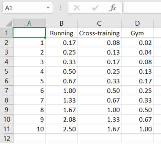
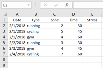
Suppose this table is placed on Sheet 1, and your table where you are inputting the data is on Sheet 2:
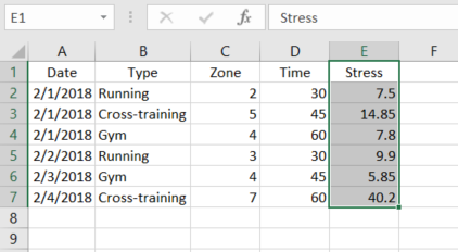
Then please enter the following formula into cell E2 in the table on Sheet 2:
=INDEX(Sheet1!$A$1:$D$11, MATCH(C2,Sheet1!$A$1:$A$11,0), MATCH(B2,Sheet1!$A$1:$D$1,0))*D2
You’ll get the total training stress for a particular activity type:
If you want to get the stress summary by date, then please use the standard Excel Subtotal feature (Data -> Subtotal).
You can find more information about INDEX and MATCH in this article on our blog. To see how to use the Excel Subtotal feature, please go here.
I hope this information will be helpful for you.
Good day. Can some assist. which function is used to auto fill these sheet on the dates side. I need short cut on my excel to auto fill the dates like that I only know control D which is time consuming.
25-Oct-17 Stopped 1203
25-Oct-17 Stopped 1203
25-Oct-17 Stopped 1203
25-Oct-17 Stopped 1203
26-Oct-17 Stopped 1203
26-Oct-17 Stopped 1203
26-Oct-17 Stopped 1203
26-Oct-17 Stopped 1203
27-Oct-17 Stopped 1203
Stopped 1203
Stopped 1203
Stopped 1203
28-Oct-17 Stopped 1203
Stopped 1203
Stopped 1203
Stopped 1203
Stopped 1203
29-Oct-17 Stopped 1203
Stopped 18
Stopped 3001
Stopped 3010
30-Oct-17 Stopped 18
Stopped 3001
Stopped 3010
Stopped 3011
Stopped 3012
Hello,
We have another article that describes how to fill empty cells in your table. Please have a look at it.
Hope you’ll find it helpful.
There is a mistake made in the post. The * is not the logical AND operator when used in array functions. It is simply that the Boolean values when used in arithmetic operators are automatically converted to numeric equivalents. So the section on AND and OR functions is wrong. Take for example the following formula presented in that section:
=SUM((A2:A9="Mike") * ( B2:B9="Apples") * ( C2:C9))
The "A2:A9="Mike"" returns a Boolean which is then converted to a numeric when it is multiplied with "B2:B9="Apples"" which in return is multiplied to "C2:C9". When both "A2:A9="Mike"" and "B2:B9="Apples"" are true, the corresponding value from "C2:C9" is taken into the sum calculation. The expression looks as follows 1*1*C.
Hello Kuze,
It is true that when the logical values of TRUE and FALSE are used in arithmetic operations, they are converted to 1 and 0, respectively. But it is also true that in array formulas, multiplication acts as the logical AND function because it follows the same rules as the AND operator. That is, multiplication returns TRUE (1) only when all of the elements are TRUE. If any of the elements is FALSE (0), the result is FALSE (because multiplying by 0 always gives zero).
On the other hand, addition acts as the OR operator because it returns TRUE (>0) if any of the elements is TRUE. And the result is FALSE (0) only when all elements are FALSE.
how to give an array as input?
just name a range, and use the range name as input.
In the first example you say the grand total can be calculated with "=SUM(B2:B6*C2:C6)" but this should actually be "=SUMPRODUCT(B2:B6*C2:C6)"
Hi Dutch,
This can actually be either, array SUM or SUMPRODUCT, which is an array formula by its nature.
Need Help
Hi am trying to use vlookup to extract muitiple column details for multiple id using array concept but am just able to extract the 1st required column details.
Here is the formula:
{=VLOOKUP(I3:I11,$A$1:$G$278,{2,3,4,5},0)}
help me to identify where am going wrong
Hi amrutha,
Please show us how your data looks like.