In this tutorial, you will lean a quick way to calculate percentages in Excel, find the basic percentage formula and a few more formulas for calculating percentage increase, percent of total and more.
Calculating percentage is useful in many areas of life, whether it is restaurant tipping, reseller commission, your income tax or interest rate. Say, you've been lucky enough to get a 25% off promotion code on a new plasma TV. Is this a good deal? And how much will you eventually have to pay?
In this tutorial, we are going to explore a few techniques that will help you efficiently calculate percent in Excel and learn the basic percentage formulas that will take the guesswork out of your calculations.
Percentage basics
The term "per cent" is derived from the Latin per centum, meaning "by the hundred". As you probably remember from high school math class, a percentage is a fraction of 100 that is calculated by dividing the numerator by the denominator and multiplying the result by 100.
The basic percentage formula is as follows:
For example, if you had 20 apples and you gave 5 to your friends, how much did you give, percentage wise? By performing a simple calculation =5/20*100 you get the answer - 25%.
This is how you normally calculate percentages in school and everyday life. Computing percentage in Microsoft Excel is even easier since Excel performs some operations for you automatically, in the background.
Regrettably, there is no universal Excel formula for percentage that would cover all possible scenarios. If you ask someone "Which percent formula do I use to get the result I want?", most likely, you will get an answer like "Well, that depends on what exactly result you want to achieve."
So, let me show you a few simple formulas for calculating a percent in Excel such as a percentage increase formula, a formula to get percentages of a total and more.
Basic Excel percentage formula
The basic formula to calculate percentage in Excel is this:
If you compare it to the basic math formula for percentage, you will notice that Excel's percentage formula lacks the *100 part. When calculating a percent in Excel, you do not have to multiply the resulting fraction by 100 since Excel does this automatically when the Percentage format is applied to a cell.
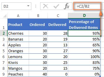
And now, let's see how you can use the Excel percentage formula on real-life data. Suppose, you have the number of "Ordered items" in column B and "Delivered items" in column C. To find out the percentage of delivered products, perform the following steps:
- Enter the formula
=C2/B2in cell D2, and copy it down to as many rows as you need. - Click the Percent Style button (Home tab > Number group) to display the resulting decimal fractions as percentages.
- Remember to increase the number of decimal places if needed, as explained in Percentage tips.
- Done! : )
The same sequence of steps shall be performed when using any other percentage formula in Excel.
In the following example, column D displays a rounded percent of delivered items, without any decimal places showing.
Calculating percentage of total in Excel
In fact, the above example is a particular case of calculating percentages of a total. Now, let's investigate a few more examples that will help you make quick work of calculating a percent of a total in Excel on different data sets.
Example 1. The total is at the end of the table in a certain cell
A very common scenario is when you have a total in a single cell at the end of a table. In this case, the percentage formula will be similar to the one we've just discussed with the only difference that a cell reference in the denominator is an absolute reference (with $).The dollar sign fixes the reference to a given cell, so that it never changes no matter where the formula is copied.
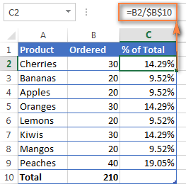
For example, if you have some values in column B and their total in cell B10, you'd use the following formula to calculate percentages of the total:
=B2/$B$10
You use a relative cell reference to cell B2 because you want it to get changed when you copy the formula to other cells of column B. But you enter $B$10 as an absolute cell reference because you want to leave the denominator fixed on B10 when auto-filling the formula down to row 9.
Tip. To make the denominator an absolute reference, either type the dollar sign ($) manually or click the cell reference in the formula bar and press F4.
The screenshot below demonstrates the results returned by the formula, the Percentages of Total column is formatted as percentage with 2 decimal places showing.
Example 2. Parts of the total are in multiple rows
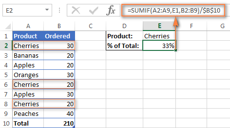
In the above example, suppose you have several rows for the same product and you want to know what part of the total is made by all orders of that particular product.
In this case, you can use the SUMIF function to add up all numbers relating to a given product first, and then divide that number by the total, like this:
=SUMIF(range, criteria, sum_range) / total
Given that column A contains all product names, column B lists corresponding quantities, cell E1 is the name of the product you are interested in, and the total is in cell B10, your real-life formula may look similar to this:
=SUMIF(A2:A9 ,E1, B2:B9) / $B$10
Naturally, you can put the product name directly in the formula, like this:
=SUMIF(A2:A9, "cherries", B2:B9) / $B$10
If you want to find out what part of the total a few different products make, add up the results returned by several SUMIF functions, and then divide that number by the total. For example, the following formula calculates the percent of cherries and apples:
=(SUMIF(A2:A9, "cherries", B2:B9) + SUMIF(A2:A9, "apples", B2:B9)) / $B$10
For more information about the SUM function, please check out the following tutorials:
Tip. In Excel 365 you can calculate percentage of total using the new PERCENTOF function.
How to calculate percent difference in Excel
Of all formulas for calculating percentage in Excel, a percent change formula is probably the one you would use most often.
Excel formula for percent increase / decrease
To calculate the percentage of difference between two values A and B, the generic formula is:
When applying this formula to real data, it is important that you correctly determine which value is A and which is B. For example, yesterday you had 80 apples and how you have 100, meaning that now you have 20 apples more than before, which is 25% increase. If you had 100 apples and now you have 80, your number of apples has reduced by 20, which is 20% decrease.
Considering the above, our Excel formula for percentage change takes the following shape:
And now, let's see how you can use this formula for calculating percent difference in your spreadsheets.
Example 1. Calculating percent difference between 2 columns
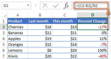
Suppose you have the last month prices in column B and this month prices in column C. Then your percent change formula takes this form:
=(C2-B2)/B2
To calculate the percent difference between two numbers correctly, carry out these steps.
- Enter the formula in any blank cell in row 2, say D2. This will output the result as a decimal number.
- Select the formula cell and click the Percent Style button on the Home tab to convert the decimal number to percentage.
- Drag the formula down to copy it to the below cells.
As the result, the formula calculates the percentage of change in this month (column C) comparted to last month (column B). Positive percentages that show percentage increase are formatted in usual black, while negative percentages (percent decrease) are formatted in red. To have this done automatically, set up a custom format for negative percentages as explained in this tip.
Example 2. Calculating percentage difference between two numbers
In case you have one column of numbers, say column C that lists weekly or monthly sales, you can calculate the percentage change between the previous week/month and the current one using this formula:
=(C3-C2)/C2
Where C2 and C3 are the numbers you are comparing.
Note. Please pay attention that you should skip the first row with data and put your percent difference formula in the 2nd cell, which is D3 in this example.
To display decimals as percentages, apply the percent format to the cells containing your formula, and you will get the following result:
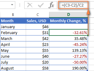
To calculate the percentage of change between a certain number and all other numbers, fix the address of that cell by using the $ sign, e.g. $C$2.
For instance, to calculates the percent increase / decrease for each month compared to January (C2), the formula in D3 is:
=(C3-$C$2)/$C$2
When copying the formula to the below cells, the absolute reference ($C$2) will remain the same, while the relative reference (C3) will change to C4, C5, and so on based on a relative position of the row where the formula is copied.
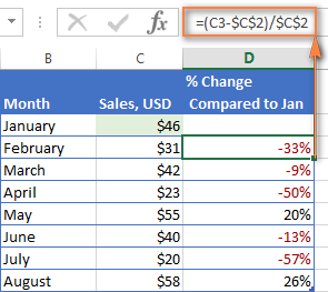
For more formula examples, please see How to calculate percentage change in Excel.
Calculating amount and total by percentage
As you've just seen, calculating percentages in Excel is easy, and so is calculating amounts and totals if you know the percentage.
Example 1. Calculate amount by total and percentage
Suppose you are buying a new laptop for $950 and they charge 11% VAT on this purchase. The question is - how much do you have to pay on top of the net price? In other words, what is 11% of $950?
The following formula will help:
Assuming that the total value is in cell A2 and percent in B2, the above formula turns into a simple =A2*B2 and returns 104.50.
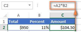
Remember, when you type a number followed by the percent sign (%) in Excel, the number is interpreted as a hundredth of its value. For example, 11% is actually stored as 0.11 and Excel uses this underlying value in all formulas and calculations.
In other words, the formula =A2*11% is equivalent to =A2*0.11. Naturally, you are free to use the decimal number corresponding to the percentage directly in a formula if this works better for your worksheets.
Example 2. Calculating total by amount and percentage
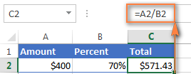
For example, you friend offered you his old computer for $400, which is 30% off the original price. You want to know what the original price was.
Since 30% is the discount, you deduct it from 100% first to know what percentage you actually have to pay (100% - 30% = 70%). Now you need the formula to calculate the original price, i.e. to find the number whose 70% equals 400.
The formula goes as follows:
Applied to real data, it may take any of the following shapes:
=A2/B2
or
=A2/0.7
or
=A2/70%
Tip. To get an answer to a more difficult question - how to calculate the interest amount of a loan payment knowing an interest rate - check out the IPMT function.
How to increase / decrease a number by percentage
The holiday season is upon us and this indicates a change in your usual weekly spendings. You may want to consider different options to find out your optimum weekly allowance.
To increase an amount by a percentage, use this formula:
For example, to increase the value in cell A1 by 20%, the formula is:
=A1*(1+20%)
To decrease an amount by a percentage:
For instance, to reduce the value in cell A1 by 20%, the formula is:
=A1*(1-20%)
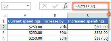
In our example, if A2 is your current expenditures and B2 is the percentage you want to increase or reduce that amount by, here are the formulas you'd enter in cell C2:
Increase by percentage:
=A2*(1+B2)
Reduce by percentage:
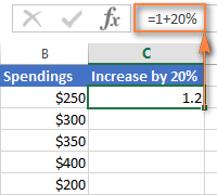
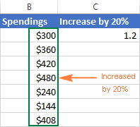
Suppose, you have a column of numbers that you want to increase or reduce by a certain percent, and you want to have the updated numbers in the same column rather than add a new column with the formula. Here are 5 quick steps to handle this task: Increase by percentage: Reduce by percentage: Naturally, you are free to replace 20% in the above formulas with the percentage you want. And here's the result - all the numbers in column B are increased by 20%:
In the same fashion, you can multiply or divide a column of numbers by a certain percentage. Simply enter the desired percentage in an empty cell and follow the steps above.=A2*(1-B2)
How to increase / reduce an entire column by a percentage
=1+20%=1-20%
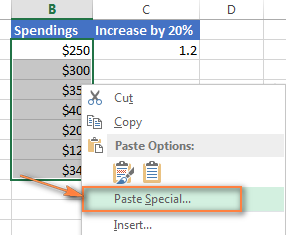
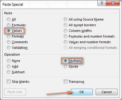
This is how you calculate percentage in Excel. And even if working with percentages has never been your favorite kind of math, by using these basic percentage formulas you can get Excel to do the work for you. That's all for today, thank you for reading!
 by
by
342 comments
I am trying to add a formula in Column C to add 9.9% to Column B.
Hi! Pay attention to the following paragraph of the article above: Increase / decrease a number by percent
Hi I have a number say 41.73 I know that this number is 20% of another number. How do I use excel to calculate what that number is 20% of?
Hi! This is a standard percentage calculation that can be performed without Excel. Divide your number by percentage (20) and then multiply by 100. Example in Excel:
=A1/20*100
Below is a snippet. What percentage is 85% based on the percentages in the table. Looking to put the percentage in B4 and then use B4 to calculate D4.
Minimum 50.00% 0.00% $110
Target 100.00% 50.00% $220
Maximum 200.00% 100.00% $439
Actual 85.00% $-
Hi! This information is not enough to guess what result you want in D4. Write what kind of result you have in mind and how you would calculate it. Then I will try to suggest a formula.
Maybe this article will be helpful: Nested IF in Excel – formula with multiple conditions.
Hi Boss,
How can I use formula to calculate percentage and text together like 20 % up or down
Hi! Extract the number of percentages from the text string. You can use these instructions for your data: Get number from the left of a string.
LEFT(A1, MATCH(FALSE, ISNUMBER(MID(A1, ROW(INDIRECT("1:"&LEN(A1)+1)), 1) *1), 0) -1)
Determine whether the word in the text is "up" or "down.
You can find the examples and detailed instructions here: Excel IF statement for partial text match (wildcard).
The formula might look like this:
=IF(COUNTIF(A1,"*up*"), B1*(100+LEFT(A1, MATCH(FALSE, ISNUMBER(MID(A1, ROW(INDIRECT("1:"&LEN(A1)+1)), 1) *1), 0) -1))/100, B1*(100-LEFT(A1, MATCH(FALSE, ISNUMBER(MID(A1, ROW(INDIRECT("1:"&LEN(A1)+1)), 1) *1), 0) -1))/100)
Hello!
I've got a tricky question which I cannot find an answer for!
I have three targets for each person, and they have to do a certain amount for each target. Two of the targets require 2 to be done, the other is only 1, and they fill out how many they have done on a spreadsheet in three separate cells (one cell for each target).
I'm trying to get excel to calculate a percentage for each person but I cannot work out the formula to give me an accurate result.
For example:
The first target may be 1 out of the 2 done (1 is written in cell E6, F6 has 2 for the target). The second target is 1 out of 1 done (1 is written in cell G6, H6 has 1 for the target). The third target is 1 out of 2 done (1 is written in cell I6, j6 has 2 for the target). The percentage should be 60% in cell K6 but the closest I've got is cell K6 displaying 66.67%.
Is there a way to get K6 to show 60%?
Thank you for any assistance you could provide!
Hello Chris!
If I understand your task correctly, the following formula should work for you:
=(E6+G6+I6)/(F6+H6+J6)
Hi Alex!
I'm definitely saving that formula for a future date!
Thank you very much for your help!
Hi again,
You can ignore this question, I finally figured out a solution to it! Turns out I just had to leave the problem in order to get my aha moment!
I have below criteria and need calculate the percentage
60-0%
Is this formula correct
=IF(I23=30,"75%",IF(I23>=45,"50%",IF(I23>=60,"0%"))))
Hi! Your formula returns text, not percentages. If you want to get a percentage depending on the condition, don't use quotation marks. Also start with the condition with the highest number. For example:
=IF(I23>=60,0%,IF(I23>=45,50%,IF(I23=30,75%)))
You can find the examples and detailed instructions here: Nested IF in Excel – formula with multiple conditions.
Hi, I am a teacher at an institution with a new set of students every month, with tests at the end of each month. There are 8 individual tests they need to take up on examination day. I would like to get a running total as well as a running percentage value based on the tests that they have taken thus far. I need this running update so that I can identify the abjectly poorer ones midway and prevent them from taking up the later set of tests if I know they will not meet the pass criteria.
For example, lets say test 1 is for 10 marks, test 2 for 20, test 3 for 30, test 4 for 40, and then repeat till we get 8 tests, amounting to a total of 200 marks.
Lets say the students have taken up 2 tests so far, I would like to obtain the total and relative total percentage value of the tests taken up till now. So I would like to know their total out of 30, as well as their percentage out of 30.
And if I enter the results for test 3, it should automatically show me their totals out of 60, as well as their percentages out of 60.
And once they take up test 4, it should automatically calculate for 100, so on and so forth till all 8 tests are done.
For reference, each test is written in a new column from A-->H, and each student occupies a new row 1-->infinity.
I hope to receive a positive reply that solves my problem. Looking forward to it eagerly.
Thank you!
Hi! If I understand your task correctly, try the following formula:
=SUM(A1:H1)/CHOOSE(COUNT(A1:H1),10,30,60,100,110,130,160,200)
The COUNT function can be used to determine the number of tests completed. CHOOSE function can be used to return the number of marks for any given number of tests. Find the sum of the scores for the completed tests using the SUM function and divide by the number of scores for those tests.
Set the cell with the formula to a percentage number format.
I need formula for percentage rent calculations for gross sales.
Base rent plus percentage of sales with breakpoints.
Sales $0-$800,000.00 pay 7%
Sales 800,000.01-1,300,000.00 pay 3%
Sales 1,300,000.01 - infinity pay 1.5%
Sales were 934,000, they should pay 7% on first 800,000 and pay 3% on the $134,000 additional. I need this formula for my spreadsheet for all months. Helpppppp
Hi! If I understand your task correctly, try to use nested IF formula:
=IF(A1<=800000, A1*0.07, IF(A1<=1300000, (800000*0.07) + ((A1-800000)*0.03), (800000*0.07) + ((1300000-800000)*0.03) + ((A1-1300000)*0.015)))
A1 represents the cell containing the total sales amount (934000 in your example).
The formula uses nested IF statements to check which tier the sales fall into:
Tier 1 (7%): If the sales (A1) are less than or equal to 800000, it simply multiplies the sales by 7% (0.07).
Tier 2 (3%): If the sales (A1) are greater than 800000 but less than or equal to 1300000, it calculates the rent in two parts:
Rent on the first 800000: 800000 * 7%
Rent on the exceeding amount (sales - 800000) at 3%.
Tier 3 (1.5%): If the sales (A1) exceed 1300000, it calculates the rent in three parts:
Rent on the first 800000: 800000 * 7%
Rent on the second tier (1300000 - 800000) at 3%
Rent on the exceeding amount (sales - 1300000) at 1.5%.
Hello...
I have 30,000 rows of data and 3 columns (Actual premium, Risk premium, Commission). The Actual premiums per row are not the same - they are all different individuals. The Risk premium is a percentage of the Actual premium and the Commission is a percentage of the Actual premium. The Risk % and the Commission % together must be 100% based on the Actual premium amount.
I have to add a formula that calculates each row with the % showing in the Risk and the Commission columns per row for that individual.
Then I have to add a formula in a single empty cell at the top of the Risk premium column and one at the top of the Commission column. These two formulas must be able to change the whole column of Risk % and the same with the Commission %. In other words, If the Risk premium is 90% and the Commission 10% I must be able to only type 90 in the Risk formula cell and 10 in the Commission formula cell for the formula to automatically update all 30 000 rows with different percentages derived from the Actual premium column per row of individual data.
How will I manage to do that? If you can assist I will sincerely appreciate it. Must hand in this spreadsheet by tomorrow and I am struggling now for days on end without success! Hope my explanation is understandable.
Hi! To use the Risk % value in all formulas in column B, write it in cell B1 and use an absolute reference to that cell in the formulas in column B.
Try to enter the following formula in cell B2 and then copy it down along the column: =A2*$B$1
If I understand your task correctly, this article may be helpful: Relative and absolute cell reference: why use $ in Excel formula
Hi I really hope someone can help.
I want to calculate that out of 1050 is the total and need to know how many tasks i have done this week and last week and then know how much is left in procentage.
Example:
Last week 500 task out of 1050 is complete
This week 670 tasks out of 1050 is complete.
Then i need to know how much in % is left before i reach the goal of 1050
If this could be used in a way for a dynamic diagram, that would be great.
I hope someone can help
i've tried reading the article but i cant figure out which one to use.
Hi! You can count the number of tasks per week using the COUNTIF function. Read more here: Using Excel COUNTIF function with dates.
This article is good.
I am n educator. I have a list of (raw) scores eg. 5, 3, 7, 1, 9. The possible total is 10.
I need a formula that will calculate
1) The percentage of each score
2) The number of scores that are LESS than 40%
I've managed to find a formula that will show how many scores are below 4, but I need to find a way to first calculate the percentage without having to insert an separate column for the percentage.
=COUNTIF(C2:C8,"<4")
Thank you
Hi!
To calculate the percentage, divide by the number of all scores. Please read the above article carefully.
=COUNTIF(C2:C8,"<4")/COUNT(C2:C8)
Hello,
I am looking to get a work load / utilization percentage formula depending how many tasks certain employees are assigned to. I have a list of names of all the employees in column M (drop down menu). I am looking to find, how many times they come up within that column and what percent of utilization they are at depending on how many assignments there are assigned to and display that in column P.
Hi!
You can count the number of tasks of each employee using the COUNIF function. There is not enough information to answer your other questions.
Hello, I am looking to get the percentage of a product(s) that was allocated to specific companies in a range of weeks, and then comparing to other range of weeks to know which products in difference were allocated. I have my worksheet set up in the following manner:
The Product and Companies are in Columns (each Company has its respective product) and in the rows I have the weeks and value allocated to each. I need to find the % certain products were allocated.
I hope I was able to explain it. Thank you for your help.
Hello!
To find the percentage, you must first find the amount for the company. To do this, you can use this guide: Excel SUMIFS and SUMIF with multiple criteria.
Hello. I am making a simple spreadsheet to enable me to quote customers. I have it laid out as follows:
In column A: Column B will hold the variable information, eg:
A1: Quantity B1: 1.000
A2: Our buying price B2: 110.00
A3: Margin (in %) B3: 81.82%
A4: Our selling price B4: 200.00
A5: Margin (£'s) B5: £90.00
I have set this up so that B3 is automatically calculated based on the contents of B2 and B4. That is: B3=(B4-B2)/B2*100
I am having to put the selling price in first, in order to calculate the margin percentage.
However! I would also like to be able to enter the margin percentage (B3) first, and have it generate my selling price (B4), based on cost price (B2). But I can't figure out how to do this.
In other words, I would like it to perform both operations: Allow me to manually enter our selling price, and automatically show me margin %, and vice versa - allow me to manually enter a margin %, and automatically show me the selling price.
Is this something anybody can help with?
Thanks in advance!
Hi!
You cannot perform these two operations at the same time using the usual Excel tools, since you cannot write a value and a formula in a cell at the same time. Your task can be accomplished with a VBA macro.
Hi, looking for help attempting to calculate % total from two filters (texts) I am using within my column.
It's for my work to know how many colleagues are using annual leave and flexi days combined.
Along top Row of my excel is Monday to Sunday and columns the name of colleagues.
I want to know at the bottom of the Columns how many people are on Annual Leave and Flexi days using a % for that day of total workforce.
My filters contain start times, finish times, Annual Leave, Flexi and Finish Times etc.
Thanks
Derrick
Hello!
To count the number of values by multiple criteria, use the COUNTIFS function. Here is the article that may be helpful to you: How to use Excel COUNTIFS and COUNTIF with multiple criteria.
I hope I answered your question. If you have any other questions, please don’t hesitate to ask.
Hello, I have two rows, one row says 10, 20, 30, 50, 100, which represent deposit amounts. Below this row shows percentage of the deposits made by customer: for ex. particular customer deposited 5 times, 3 out of which was 10$, so he places 10$ most frequently. Now I want a formula to give me number with the highest percentage below. I mean the formula which will give me number 10. I hope I managed to explain.
Hello!
If I understand your task correctly, find the maximum number using the MAX function. Find the position of this number and extract the corresponding value with INDEX MATCH functions.
=INDEX(A1:E1,MATCH(MAX(A2:E2),A2:E2,0))
I hope my advice will help you solve your task.
Thank u very much.
Hi, if I have 10 columns of numbers together with 1 column indicating the total number of the 10 added up, is there a faster way to find the percentage of each over the total sum? Hope to get help as I have many % to be counted over the total sum.. Thank you.
Hello!
If you need to divide many cells by the same number, then use these recommendations: How to copy formula without changing references. Hope this is what you need.
Hi, I would like to build an excel for different pourcentages applied to a different range of value:
If 0 to 55000 apply 0.5%
55,000.01 to 25000 apply 1%
250,000.01 to 400000 apply 1.5%
400,000.01 to $2,000,000.00 apply 2%
if over $2,000,000: apply 2.5%
How can i do that properly?
Thank you!
Hi!
You can find the answer to your question in the first paragraph of this article - Excel Nested IF statements - examples, best practices and alternatives.
Hi thank you very much, i tried this reading the article but it doesn't return the right pourcentage. =IF((B4=55000.01, B4=250001, B4=400001, B42000000), "")))) do you know why?
Found the solution thank you !
=IF((B4=55000.01, B4=250001, B4=400001, B42000000), ""))))
I need my excel sheet to average a set of numbers as follows: the percent of numbers at or above 70 in a single column.
For example: If my numbers in the column are- 100, 70, 20, 50, 85, 65...what is the percentage of numbers at or above 70.
I know how to calculate this by hand, but is there a way for excel to calculate this?
Hello!
You can determine the percentage of values less than 70 and greater than 70 using the FREQUENCY formula -
=FREQUENCY(A1:A10,69)/COUNT(A1:A10)
Or use COUNTIF function to count the number of values greater than 70 -
=COUNTIF(A1:A10,">=70")/COUNT(A1:A10)
I hope it’ll be helpful.
Question is:
Condition - order should be supllied within 48 hours (2 days)
Need to calculate the percentage for the amount of orders supllied within 48 hours to see if I am keeping the markup of 90%. Can I know what is the formula to get the calculations between the ordered date and date received with the number of orders.
Hi!
If you have a column in which the supllied time is calculated, then using the SUMIF function, you can calculate the sum of orders completed in 2 hours.
Hi! Is there a way or a formula of highlighting the values using conditional formatting per say less than 10% of the total without having to calculate the percentages beforehand and a separate row or a column for percentage?
Hi!
The following tutorial should help: Excel formulas for conditional formatting based on another cell value.
Here is an example formula:
=D2/SUM($D$2:$D$10)<0.1
I hope my advice will help you solve your task.