I this article you will learn how to count cells by color in Excel and get the sum of colored cells. These solutions work both for cells colored manually and with conditional formatting. You will also learn how to filter cells by several colors in Excel 2010, Excel 2013, Excel 2016, and Excel 2019.
If you actively use diverse fill and font colors in your Excel worksheets to differentiate between various types of cells or values, you may want to know how many cells are highlighted in a certain color. If your cells' values are numbers, you may also want to automatically calculate the sum of cells shaded with the same color, e.g. the sum of all red cells.
As all of us know, Microsoft Excel provides a variety of formulas for different purposes, and it would be logical to assume that there are some to count cells by color. But regrettably, there is no formula that would let us sum by color or count by color in a usual Excel worksheet.
Apart from using third-party add-ins, there is only one possible solution - utilize User Defined Functions. If you know very little about this technology or have never heard this term before, don't be afraid, you will not have to write the code yourself. You will find the perfect code (written by our Excel guru) here and all that you will have to do is copy / paste it into your workbook.
Suppose you have a table listing your company's orders where the cells in the Delivery column are colored based on their value - "Due in X Days" cells are orange, "Delivered" items are green and "Past Due" orders are red.
What we want now is automatically count cells by color, i.e. calculate the number of red, green and orange cells in the worksheet. As I explained above, there is no straightforward solution to this task. But luckily we have very skilled and knowledgeable Excel gurus in our team and one of them has written the faultless code for Excel 2010, 2013 and 2016. So, move on with the 5 quick steps below and you will know the number and sum of your color cells in a few minutes.
Function GetCellColor(xlRange As Range) Dim indRow, indColumn As Long Dim arResults() Application.Volatile If xlRange Is Nothing Then Set xlRange = Application.ThisCell End If If xlRange.Count > 1 Then ReDim arResults(1 To xlRange.Rows.Count, 1 To xlRange.Columns.Count) For indRow = 1 To xlRange.Rows.Count For indColumn = 1 To xlRange.Columns.Count arResults(indRow, indColumn) = xlRange(indRow, indColumn).Interior.Color Next Next GetCellColor = arResults Else GetCellColor = xlRange.Interior.Color End If End Function Function GetCellFontColor(xlRange As Range) Dim indRow, indColumn As Long Dim arResults() Application.Volatile If xlRange Is Nothing Then Set xlRange = Application.ThisCell End If If xlRange.Count > 1 Then ReDim arResults(1 To xlRange.Rows.Count, 1 To xlRange.Columns.Count) For indRow = 1 To xlRange.Rows.Count For indColumn = 1 To xlRange.Columns.Count arResults(indRow, indColumn) = xlRange(indRow, indColumn).Font.Color Next Next GetCellFontColor = arResults Else GetCellFontColor = xlRange.Font.Color End If End Function Function CountCellsByColor(rData As Range, cellRefColor As Range) As Long Dim indRefColor As Long Dim cellCurrent As Range Dim cntRes As Long Application.Volatile cntRes = 0 indRefColor = cellRefColor.Cells(1, 1).Interior.Color For Each cellCurrent In rData If indRefColor = cellCurrent.Interior.Color Then cntRes = cntRes + 1 End If Next cellCurrent CountCellsByColor = cntRes End Function Function SumCellsByColor(rData As Range, cellRefColor As Range) Dim indRefColor As Long Dim cellCurrent As Range Dim sumRes Application.Volatile sumRes = 0 indRefColor = cellRefColor.Cells(1, 1).Interior.Color For Each cellCurrent In rData If indRefColor = cellCurrent.Interior.Color Then sumRes = WorksheetFunction.Sum(cellCurrent, sumRes) End If Next cellCurrent SumCellsByColor = sumRes End Function Function CountCellsByFontColor(rData As Range, cellRefColor As Range) As Long Dim indRefColor As Long Dim cellCurrent As Range Dim cntRes As Long Application.Volatile cntRes = 0 indRefColor = cellRefColor.Cells(1, 1).Font.Color For Each cellCurrent In rData If indRefColor = cellCurrent.Font.Color Then cntRes = cntRes + 1 End If Next cellCurrent CountCellsByFontColor = cntRes End Function Function SumCellsByFontColor(rData As Range, cellRefColor As Range) Dim indRefColor As Long Dim cellCurrent As Range Dim sumRes Application.Volatile sumRes = 0 indRefColor = cellRefColor.Cells(1, 1).Font.Color For Each cellCurrent In rData If indRefColor = cellCurrent.Font.Color Then sumRes = WorksheetFunction.Sum(cellCurrent, sumRes) End If Next cellCurrent SumCellsByFontColor = sumRes End Function
If you are not very comfortable with VBA, you can find the detailed step-by-step instructions and a handful of useful tips in this tutorial: How to insert and run VBA code in Excel.
In this example, we use the formula =CountCellsByColor(F2:F14,A17)
where F2:F14 is the range containing color-coded cells you want to count and A17 is the cell with a certain background color, a red one in our case.
In a similar way, you write the formula for the other colors you want to count, yellow and green in our table.
If you have numerical data in colored cells (e.g. the Qty. column in our table), you can add up the values based on a certain color by using an analogous SumCellsByColor function:
As demonstrated in the screenshot above, we used the formula =SumCellsByColor(D2:D14,A17)
where D2:D14 is the range and A17 is the cell with a color pattern.
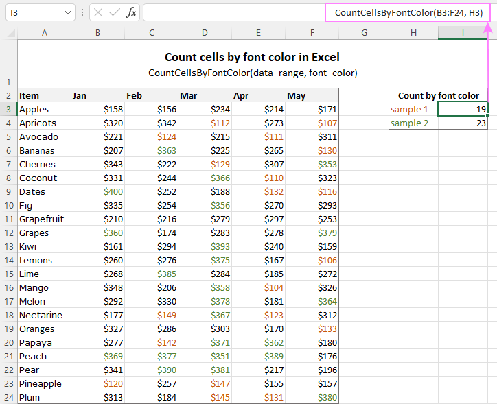
In a similar way you can count cells and sum cells' values by font color using the CountCellsByFontColor
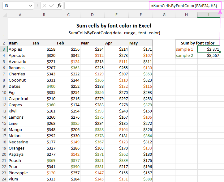
and SumCellsByFontColor
functions, respectively.
The VB script below was written in response to Connor's comment (also by our Excel's guru Alex) and does exactly what Connor requested, namely counts and sums the cells of a certain color in all worksheets of the workbook. So, here comes the code:
Function WbkCountCellsByColor(cellRefColor As Range) Dim vWbkRes Dim wshCurrent As Worksheet Application.ScreenUpdating = False Application.Calculation = xlCalculationManual vWbkRes = 0 For Each wshCurrent In Worksheets wshCurrent.Activate vWbkRes = vWbkRes + CountCellsByColor(wshCurrent.UsedRange, cellRefColor) Next Application.ScreenUpdating = True Application.Calculation = xlCalculationAutomatic WbkCountCellsByColor = vWbkRes End Function Function WbkSumCellsByColor(cellRefColor As Range) Dim vWbkRes Dim wshCurrent As Worksheet Application.ScreenUpdating = False Application.Calculation = xlCalculationManual vWbkRes = 0 For Each wshCurrent In Worksheets wshCurrent.Activate vWbkRes = vWbkRes + SumCellsByColor(wshCurrent.UsedRange, cellRefColor) Next Application.ScreenUpdating = True Application.Calculation = xlCalculationAutomatic WbkSumCellsByColor = vWbkRes End Function
You use this macro in the same manner as the previous code and output the count and sum of the colored cells with the help of the following formulas, =WbkCountCellsByColor()
and =WbkSumCellsByColor()
, respectively. Simply enter either formula in any empty cell on any sheet without defining a range, specify the address of any cell of the needed color in brackets, e.g. =WbkSumCellsByColor(A1), and the formula will display the sum of all the cells shaded with the same color in your workbook.
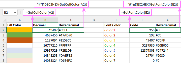
Here you will find a summary of all the functions we've used in this example as well as a couple of new ones that retrieve color codes.
CountCellsByColor(range, color code)
- counts cells with the specified background color.
In the above example, we used the following formula to count cells by color =CountCellsByColor(F2:F14,A17) where F2:F14 is the selected range and A17 is the cell with the needed background color. You can use all other formulas listed below in a similar way.
CountCellsByFontColor(range, color code)
- counts cells with the specified font color.SumCellsByColor(range, color code)
- calculates the sum of cells with a certain background color.SumCellsByFontColor(range, color code)
- calculates the sum of cells with a certain font color.GetCellFontColor(cell)
- returns the color code of the font color of a specified cell.GetCellColor(cell)
- returns the color code of the background color of a specified cell.Well, counting cells based on color and getting the sum of colored cells was pretty easy, wasn't it? Of course if you have that little VBA gem that makes the magic happen : ) But what if you do not color cells manually and rather use conditional formatting, as we discussed in these two articles How to change the background color of cells and How to change a row's color based on cell value?
If you have applied conditional formatting to color cells based on their values and now you want to count cells by color or sum the values in colored cells, I have bad news - there is no universal user-defined function that would sum by color or count color cells and output the resulting numbers directly in the specified cells. At least, I am not aware of any such function, alas : (
Of course, you can find tons of VBA code on the Internet that attempts to do this, but all those codes (at least the examples I've come across, do not process conditional formatting such as "Format all cells based on their values", "Format only top or bottom ranked values", "Format only values that are above or below average", "Format only unique or duplicate values". Besides that nearly all those VBA codes have a number of specificities and limitations because of which they may not work correctly with certain workbooks or data types. All in all, you can try your luck and google for an ideal solution and if you happen to find one, please do come back and post your finding here!
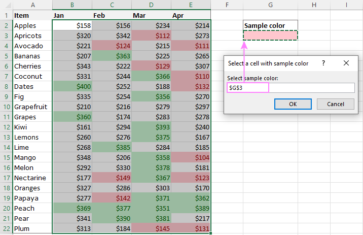
The VBA code below overcomes the above mentioned limitations and works in Microsoft Excel 2010, Excel 2013 and Excel 2016 spreadsheets with all types of condition formatting (kudos to Alex again!). As a result, it displays the number of colored cells and the sum of values in those cells, no matter which type of conditional formats are used in a sheet.
Sub SumCountByConditionalFormat() Dim indRefColor As Long Dim cellCurrent As Range Dim cntRes As Long Dim sumRes Dim cntCells As Long Dim indCurCell As Long cntRes = 0 sumRes = 0 cntCells = Selection.CountLarge indRefColor = ActiveCell.DisplayFormat.Interior.Color For indCurCell = 1 To (cntCells - 1) If indRefColor = Selection(indCurCell).DisplayFormat.Interior.Color Then cntRes = cntRes + 1 sumRes = WorksheetFunction.Sum(Selection(indCurCell), sumRes) End If Next MsgBox "Count=" & cntRes & vbCrLf & "Sum= " & sumRes & vbCrLf & vbCrLf & _ "Color=" & Left("000000", 6 - Len(Hex(indRefColor))) & _ Hex(indRefColor) & vbCrLf, , "Count & Sum by Conditional Format color" End Sub
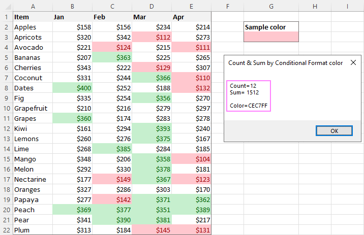
As a result, you will see the following message:
For this example, we selected the Qty. column and got the following numbers:
If you have any difficulties with adding the scripts to your Excel workbooks, such as compilation errors, formulas not working and so on, please download this sample workbook with the CountCellsByColor and SumCellsByColor functions ready for use and try them on your data.
Updated on 1-Jul-2014
When we published this article, we hoped it would be popular because we used to get a lot of questions about how to count and sum cells by color in Excel. But even in our wildest expectations, we did not think it was going to be that popular! What you see in comments on this page is just a tiny portion of the enormous feedback we have received. So, our team decided to take a step further and create an Excel add-in that would count and sum cells by the color you specify or by all colors in the selected range.
Let me introduce you to our brand new tool - Count & Sum by Color for Excel 2019 - 2007. Once installed, it will place 2 buttons onto the Ablebits Data tab on your Excel ribbon - One Color and All Colors, as you can see in the screenshot below:
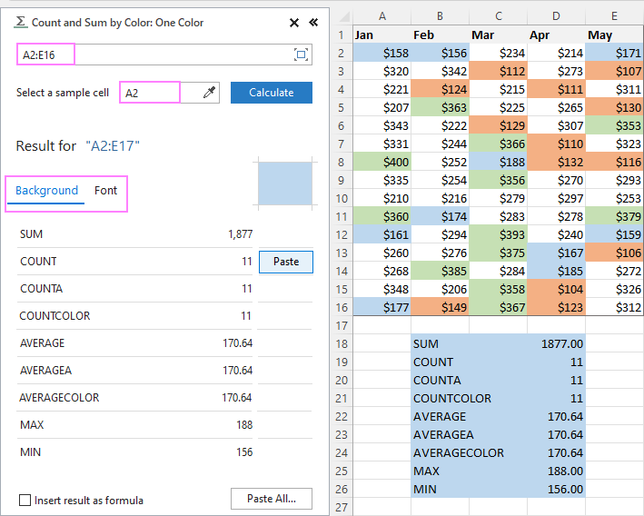
You simply click the One Color button on the ribbon and have the Count & Sum by Color pane open at the left of the worksheet. On the pane, you select:
Once done, click Calculate and see the result in the lower part of the pane straight away! Apart from the count and sum, the add-in calculates the average and finds the max and min values. No macros, no formulas, no pain :)
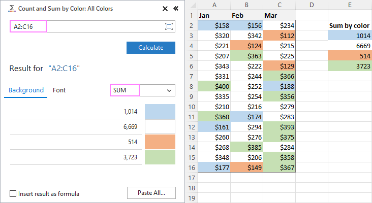
The All Colors option works basically in the same way, except that you do not have to choose the color. In the "Show results for" section, you can select any of the following options: Count, Sum, Average, Maximum or Minimum value.
If you want to copy the results to your worksheet, click the Paste results... button at the bottom of the Count & Sum by Color pane.
And here is a list of the main features you will find in the Count & Sum by Color add-in:
Currently the add-in is available as part of the Ultimate Suite for Excel. This is a collection of our best tools especially designed to deal with the most tedious, painstaking and error-prone tasks in Excel.
In addition to the Count & Sum by Color add-in, the Ultimate Suite includes over 60 time-saving tools tools that will help you merge data from different worksheets, remove duplicates, compare sheets for matches and differences, and a lot more!
If you like the tools, don't miss this special opportunity to get a license at the lowest price:
576 responses to "How to count and sum cells by color in Excel"
frist of all thank u for this good data
but if i change any color in range it doesn’t be counted and the result didn’t updated? i want to count cells by color even i change the color in the range
Ahmed; taken from the article
"Note: If after applying the above mentioned VBA code you would need to color a few more cells manually, the sum and count of the colored cells won't get recalculated automatically to reflect the changes... simply place the cursor to any cell and press F2 and Enter, the sum and count will get updated. The same applies to the other macros you will find further in this article."
Very helpful. thank you.
Hi,
I have data where i need to insert sum formula for perticular font coloure rows to sum its above data till the coloure change.
please help me with suitable macro or formula.
Is there a way to use the countcellsbycolor function on a filtered data set? (excluding the hidden data)
Try subtotal function.
functions are not working on conditional formation
I am having the same issue
Very helpful, great instruction!! Thank you.
Function works great - just not on cells using conditional formation.
Is there way to count cells by colour if the colour is assigned by conditional formatting?
superb
i want to know how to autocount all the numbers insid the color cells
So legit I actually took a moment to thank you for this little piece. Just what I needed!
The count cells by conditional format is fantastic. I have been searching the web for over a year for a good solution. I have another twist to this. I have a very large data set that should be unique numbers. I can set a conditional format to look for duplicates but then I need to find them, if they exist. Is it possible to adapt the code to find the first cell that is conditionally formatted (if there is one) and then use this cell to set the format to count possible additional entries in the entire dataset?
Good article.....Keep going
super helpful and very quick to apply! Thanks.
Doesn't work. Just keep saying 0. followed everything, word for word. The file is even saved as macro ready. Even played with the formatting to match what I was looking for. Nada. I spent over an hour trying to figure out why. I went as far as using a new workbook completely empty starting from scratch to see where I went wrong. Still nothing. I can't figure this out. I'll keep looking online.
Hi, I would like to count cell color of individual worksheet on a master sheet. Each worksheet must be separate.
Hi,
Thank you for the codes.
I have used the code for the count by conditionally formatted color, and it works. But rather than the information being shown in a message box, I want the information to appear on a cell. Is this possible? Can I amend the code in a way to accommodate this?
How were you able to count by conditionally formatted colour cells? I've been struggling with me returns!
Hello, Khalid.
It looks like our Count and Sum by Color add-in can help you with your task. The tool can help you sum and counts cells by font or background color in a few clicks. If you want to see how the Count and Sum by Color add-in works, feel free to install the fully functional 14-day trial version of Ultimate Suite that contains all our products for Excel (60+ add-ins) using this direct download link.
After installation you can find the add-in in the Calculate group under the Ablebits Tools tab. If you need the instructions how to use the add-in, you can find them on its help page.
Don't hesitate to contact us again if you have any questions or need further assistance.
Hi Svetlana,
Wonderful code, working perfectly! I just found one issue - when I delete something or leave an empty cell within the region it is still counted by CountCellsByFontColor.
Any idea how to overcome this? How can I count only non-empty cells based on the font color
Thanks,
Hi
Your code works perfectly - thank you. I understand that you can't create a function that will count cells for all types of conditional formatting and output the results to a cell. But if you were to constrain so it assumes one kind of conditional formatting, would that be possible? I only ever use conditional formatting based on cell contents or formulas and I can usually choose either. Would it be possible to create a function that worked with one of those types?
Thanks
Paul
I'm getting a syntax error on "Dim indRefColor As Long".
As do I.
"Compile error:
Syntax error"
I copy-pasted the code in to my own document and I still get that error. Doesn't get it with the downloaded example document, and can't figure out what the difference is!
Hi Christopher / Anton, I believe the code in this page had some syntax issues. Please download the sample document from this page. Go to VBA module and copy-paste the code to your sheet.
Thank you!
I've just discovered your website, blog, and products. They're terrific.
Its really good but i wants to know if i change the colour then it can do auto change in sum
Hello, Rikin,
Please note that the sum and count of the colored cells won't get recalculated automatically. Once you've made all the necessary changes, simply place the cursor to any cell and press F2 and Enter, the sum and count will get updated.
Feel free to contact us again if you have any other questions.
Hi,
Is there a way to set up sumcellsbycolour so it calculates automatically? I have calculation options set up as automatic but this particular formula is not updating automatically. this formula works great otherwise.
thank you
Fiona
the closest thing I can suggest is to have VBA code that updates on selection change, more on that here https://trumpexcel.com/vba-events/#Worksheet-Change-Event
However, you have to move click the cursor somewhere before excel will recalculate
Hi,
I'm still returning #Name? after inputting the VBA into the module. It seems the sumcount via Alt+F8 seems to work, however when I try to count the conditionally formatted cells via colour it returns #Name?
Any advice or suggestions where I'm messing up?!
Thank you so much for this code!
I do not know what I would do without it!!!!
Very very helpful... once it all works out!!!
A tip that helped me (not a coder) was to know that I could click any cell that had the color I was referencing in the formula (=CountCellsByColor(range, color code) )
easy peasy!!! Thanks I will be sharing
Hello l have vertical blank spaces say 15
Then say a color (say red) that would end the blanks being counted
I then have more vertical blank spaces say 3 (3 blank spaces) in the same vertical line or drop
And then a color (say red again) to end the count and it continues
Then more blanks then ended with a red (blanks counted and ended count with another red)
Etc, etc, etc all different
I would like to sum up the blanks then number them before it moves onto the next lot of blank cells and number them also on the last blank space (or the beginning) of each lot of blank cell
In other words when it gets counted down (vertically) to the last blank cell before the color in a cell it will sum it up.
Then when I have a list of multiple blank results of the blank cells in block l want to work out the average blanks of all of them.
In other words sum up the blanks that are broken up by the reds (it could be a different colour)
Thank you
Slane
Hello, Slane,
Our technical specialist took a look at your task. Unfortunately, there is no easy way to solve it. Most likely you need a special macro. I am really sorry we can’t help you with this.
You may try to find the solution in VBA sections on mrexcel.com or excelforum.com.
Sorry for not being able to help you better at the moment.
I've set up the macro, even downloaded Kutools and nothing seems to be able to count a range of a row (D3:D15) and give me a sum of either green, yellow, or red, conditionally formatted cells based on percentages. I've spent a few hours on this now, and have to revert back to counting manually. a copy of a portion to be counted is here, and need it as the 2nd recap.
this is Jan thru Jun, all columns, but it won't paste as it looks in excel.
Jan Feb Mar Apr May Jun
103.4% 100.5% 101.8% 94.6% 99.3% 91.4%
96.0% 93.6% 92.7% 96.1% 103.0% 100.1%
77.3% 87.0% 80.7% 99.7% 94.9% 95.1%
106.4% 100.6% 107.0% 103.1% 99.0% 107.1%
91.5% 99.1% 72.8% 89.4% 106.9% 90.8%
99.0% 75.4% 84.6% 93.3% 84.5% 78.2%
my formula is this, to create the conditional format
= 98.0% through 102.0% = green
= 103-104% = yellow
= 105.0% = red
This is the recap i need to put in the macro to count whether Green, yellow, red.
Green Yellow Red
0 0
0 12 0
3 2 7
3 2 7
2 0 10
1 0 11
0 0 12
1 1 10
How to use the macro to count conditional formatted cell color in a formula, so the results show not as a comment?
I have downloaded and used the Ablebits Add-on successfully, Thank you for that. What I would like to do with that data is have it show up in a cell and be update-able. I have a spreadsheet that I am trying to count the colored cells that are out of range, I don't need an average of the cells just the number of red colored cells. I want that data to then be documented in a separate cell not just in a report on the side bar. My scenario is as follows: F5:AM5 (Conditionally Formatted to turn red if out of spec) & AO5 (Count Amount of conditionally formatted red cells out of spec)
Hello, Chad,
Thank you for contacting us and for your interest in our software.
If you mean our Count and Sum by Color tool, yes, it can count cells by font or background color, but, unfortunately, it is not possible to automatically update the result of calculation when the number of colored cells change in the current version of the add-in.
Feel free to contact us again if you have any other questions or need further assistance.
veeeeeeeeeeeeeeeeeeeeeeeeeeeeeeeeeeeeeeeery usefull
thanks lot
Thank you!!! Works like a charm on cells, except if cell contains an Array formula and cell background or font color is set via conditional formatting. In cells with Array formula it only sees all cells as having the default color.
Thank you. It is very helpful formula.
Hi, thank you, this works just as I needed it, but I now have a problem. As soon as I save the file as xlsm file and re-open the file, all the formulas give me a #NAME? error in the place of the answers. What must I do to prevent this from happening?
thank you so much, this was extremely helpful while i was creating a formulated leave planner for my account.
however, if you could help me or is there are possible way to find out how to count the number of consecutive occurrences , meaning, in a month, if an employee AWOL's on the 12th, 13th and 14th
the count will be 3 days, however, that is just 1 consecutive occurrence.
Good formula and thank you for posting it. However, I would like to modify the counting macro to only count the cells by color that have a value > 0 in them. In other words, if I have 10 cells, but only 7 of them have data entered with a value > 0, I only want the formula to return the count of 7. How would I go about doing this?
not working in row format
I have tried the F2 and Enter process but it doesn't work - it just dims the screen. Any suggestions? Thanks.
I used the instruction as give with the formula: =CountCellsByColor(B4:B69,B72)
I received the error #NAME?
When I ran Evaluate Formula function it showed #NAME?(B4:B69,B72)
So it seems that despite me pasting the functions into the Visual Basic Editor it isn't recognising the CountCellsByColor function name
Can anyone help me troubleshoot this please?
what about excel 2019???
Can I count the number of coloured cells with coloured formatting in a non consecutive range. For example if I were to wear blue socks on different days and colour the cells accordingly would I be able to count the number of times I had worn them on a particular day eg Monday.
I guess the question is how do I stipulate the range I am asking the formula to address if the cells are not adjoining
thanks.
Hello Svetlana and team.
An excellent product with superb easy to follow descriptive documentation. Thanks and well done.
Thank You so much. It works perfect. Thank you once again!
Once I save it all the figures they went to hash marks. What format do I save the counting cells as?
Great bit of code, is there any way to count the number of cells with coloured text if a cell contains two or more different colours? i have a calendar on excel with events happening per day, if there are two or more events per day then the text is coloured differently within the same cell. I am looking for the number of events per colour.
I have a sheet with numbers scattered and colors.
I want to count how many time a individual number appears with a particular color
EG how many time the number one appears with a yellow background, or reg background
How many times the nu
mber 2 appears with a yellow background or red background
Thank you very much it was really helpful. Thank you once again.
Great code and helpful for work.
I noticed that whenever I try to apply the VBA code to other workbooks (other tabs) in the same spreadsheet, I keep getting a #NAME? error. Now the error is applied to all my countcellsbycolor formulas/cells. Any help?
Hi,
I am using this function in a large table of data and I am sub-totalling by 11 colors. It works to begin with and is brilliant, but then the function keeps returning a N/A Value not available error. Do you know why? It seems unstable. I am in Excel 2016. Thanks a million. Darren
What if I want to count cell colors with multiple range & criteria? I don't see that as an option here, and i'm not a coder. Would it be simple to add an IF function to this to accomplish this task?
example: =CountCellsByColorIF($A$3:$A$12,"Yes",$B$3:$B$12,"Accepted",!A20)
IF A=True & B=True, Then Count X Color
Thank you, this is exactly what I needed!
Thank you!
HI,
This is an amazing code,but it always rounds up my numbers. Is there a way for me to have it so that it can sum by two decimal places? For Example, .05+1.2=1.25....
When I use the SumbyColor function, it does not prompt you to enter the different portions of the argument like with other functions that prompt you to put a comma which then shows you performing the other arguments.
This is really helpful. Well explained.
I am trying to write a formula to calculate a golf handicap. I use a spreadsheet that records scores each week across a line for each player. I need to use only ten of twenty scores for each player. I want to use highlight colors to identify the ten scores to use and then add them across the line of scores as well as divide the total by 10 and subtract 36. all the info I can find is about totaling columns. Is there a way to add in a line?
hi thanks for explaining this i am now a step further forward, however my sheet, i have a cell that changer color when past a certain date, when it does this i wish it to send an email to address listed on another cell (same row) with a pre set message.
is there something i can add to this?
Thank you! The very best article related to this topic. Made my day.
Hello, why diagonal border in M. Excel in conditional formatting not active, if possible review it and fix it and add it to conditional formatting
thank you
Hello!
Thanks for this amazing code!
Dear Concern
How to used your formula with one more condition suppose i have different product in one column and there cashflow in second column and if the cashflow are highlighted by different colour as deffer and advance payment now i want for a particular product what is advance and what is deferred from huge data i cant get the required result from your formulas
I am looking for a similar forumula - trying to use SUMIFS with the countcellsbycolour - did you find a solution?
Dear Concern
How to used your formula with one more condition suppose i have different product in one column and there cashflow in second column and if the cashflow are highlighted by different colour as deffer and advance payment now i want for a particular product what is advance and what is deferred from huge data i cant get the required result from your formulas
Thanks for the coding - cut my work effort in half! Is there any way that this can be implimented into a COUNTIF/COUNTIFS formula - Ive tried majority of things and im not getting any results.
The plan is that I would like to find a number based on how often one of my numbers has been highlighted through a table of alot of other numbers. I.e - say that A1 has the number in highlighted but also further along the table there is another one highlighted at J16 i would like to get a result of that.
ive tried
=COUNTIFS(Sheet1!U36:ZZ50,"15",Sheet1!U36:ZZ50,CountCellsByColor(Sheet1!U36:ZZ50,Sheet1!A16))
where am i going wrong? thankyou in advance!
Following this it would probably benefit to know my motive - i would like to know the number of time A21 (a number) comes up in the table d36:zz50 and has been marked yellow.
I need something similar did you get an answer.....?
i cant edit the file to include more colours?
I am trying to create a file that has all world countries and depending on the maual coloring, it will tell you pending countries you dont have yet. I need 7 colours, with one variant of each (light red, dark red, light orange, dark orange etc)
plz help.
I just want to say thank you for sharing you knowledge. It is very useful.
Hi - this is super useful! However is there a formula I could use to sumif the cell colour matches and the font colour matches?
Hi, Really It's very useful and color Counts, Sum by Color tool, yes, it can count cells by font or background-color Well explained. thanks a lot...
Is there a way I can sum amounts by color, but the colors are in one column and the amounts (without color) are in another column?
This is awesome. Thanks!
Love You, it's exactly what I wanted.
Hi is there a way to make the cell color range a criteria, instead of range?
Assalamualaikum Wa Rahmatullah
Thank you for such a nice post. Extremely Helpful
Best Regards
Jawad Hussain
At first the function would not work. I realized I formatted the cell as "Text." Once I changed it to "General," the formula worked! Thanks so much!
How can i give three different colours diagonally to selected multiple cells
Can I upload a picture saved from a cross stitch program that puts whatever picture I want into a graph and have it be able to tell me how many of each different color within that upload graph. If not do you know of a program that will do this
I want to return the sum in a cell for the conditional formatting VBA. How do I do that?
I am trying to save this as an addin. I declared all the functions public, but when i run the function, i always get #Value Error.
Please help!!!
When I close and open the worksheet again, It doesn't work (#Name?)
Have the same issue!
Can anybody help with this?
Hi I wanted to ask this.
Im using 3 colours for scheduling purposes
Colour Red - Whether we've been to location
Colour Blue - Person A has been to location
Colour Purple - Person B has been to location
When I wanted to calculate a single colour, it works out fine.
But if I wanted to combine both colours to be counted as one, I run into value error.
Could someone help me with this?
This is my original forumula calculating 1 colour
=COUNTCellsByColor(AJ70:BL70,$A$1)
This is what i attempted when trying to caculate both mine and my colleagues colour.
=COUNTCellsByColor(AJ70:BL70,$A$4)+(AJ70:BL70,$A$3)
Could someone help me on this?
Should I be able to install this module to my personal workbook so that I can use it for any excel spreadsheet? If so, what am I missing to get that to actually work? Since I'm trying and failing at that.
Is there a way to know how many cells I have by both the color of the cell and the font of the cell. Like if I had cells that were blue with black font and then cells that are pink with black font.
The code is great and it saves me a lot of time in working with the color-code count and sum. Thanks for the generous gem, as other said.
Thank you so much! That worked like magic!
good article, However it is not working for me.
I have a my data, I have applied a conditional formatting where any cell in that column had a value of "y" the entire row will be colored green.
Right now i have 20 rows of data, about 11 of them have "y" in Column D. i have copied the code to VBA module, but my result for color green cells is 20, not 11.
Not sure why is not working.
Help, please
Thanks so much for this! Saved me much time and effort!
HI,
I am using the conditional color code counting macro as below.
In excel 2019 I get an error "Compile error: Invalid outside procedure", can you help me to correct this error?
Thx
Ton
Sub SumCountByConditionalFormat()
Dim indRefColor As Long
Dim cellCurrent As Range
Dim cntRes As Long
Dim sumRes
Dim cntCells As Long
Dim indCurCell As Long
cntRes = 0
sumRes = 0
cntCells = Selection.CountLarge
indRefColor = ActiveCell.DisplayFormat.Interior.Color
For indCurCell = 1 To (cntCells - 1)
If indRefColor = Selection(indCurCell).DisplayFormat.Interior.Color Then
cntRes = cntRes + 1
sumRes = WorksheetFunction.Sum(Selection(indCurCell), sumRes)
End If
Next
MsgBox "Count=" & cntRes & vbCrLf & "Sum= " & sumRes & vbCrLf & vbCrLf & _
"Color=" & Left("000000", 6 - Len(Hex(indRefColor))) & _
Hex(indRefColor) & vbCrLf, , "Count & Sum by Conditional Format color"
End Sub
I have copied one of your Function formula (CountCellsByColor) and made small changes to it (see below). But when I use the formula =CountCellsByColor(A16:G16,J2) it gives me #VALUE!
(A value used in the formula is of the wrong data type). What am I doing wrong?
Function CountCellsByColor(rData As Range, cellRefColor As Range) As Long
Dim indRefColor As Long
Dim cellCurrent As Range
Dim cntRes As Long
Application.Volatile
cntRes = 0
indRefColor = cellRefColor.Cells(1, 1).DisplayFormat.Interior.Color
For Each cellCurrent In rData
If indRefColor = cellCurrent.DisplayFormat.Interior.Color Then
cntRes = cntRes + 1
End If
Next cellCurrent
CountCellsByColor = cntRes
End Function
This was a great help. Thanks so much!
i had to count colored cells in a ROW and the formula worked great, very flexible for non-vba coders! Many thanks
I keep getting an error in VBA that says:
Compile Error:
Expected: list separator or )
How do I count non-contiguous cells?
This VBA code works great, thank you for posting it. But, since my cells are conditionally colored green for the lowest sum in a range, it will not pick up on the conditional color. Any way you happen to have VBA code for conditionally colored cells?
The VBA works great, thank you for posting. How do I incorporate the GetCellColor to count cells between a date range using a =CountIfs function? I have done the following so far but its returning a zero value:
=COUNTIFS(E7:NE7, GetCellColor(NK4),E2:NE2,">="&E2,E2:NE2,"<="&TODAY())
**E7:NE7 Data Range
**NK4 cell color reference
**E2 Start Date
**NE2 End Date
Appreciate the feedback. Thanks.
Hello Jonathan!
I cannot validate the formula on your data. But something like this will work for you.
Please copy the VBA code to your workbook and then enter the following array formula (remember to press Ctrl + Shift + Enter to complete it):
=SUM((GetCellColor(E7:NE7)=GetCellColor($NK$4)) * (E2:NE2>=$E$2) * (E2:NE2<=TODAY()))
Hope this is what you need.
I have an issue I just ran into with this that was hoping to get some help on. When the cells are being colored by rules in the column, the CountCellsByColor doesn't count those. I have a reference cell that is colored the same as those in the column that I'm using. I'm just using the simple =CountCellsByColor(AE4:AE24,C25) where C25 is colored the same as some cells in AE4:AE24, but cells in that range are not manually colored, they are being determined based on rules. Any ideas?
Hello Jake!
The answer to your question is given in the article above.
Thanks so much (again), you guys are the best. Such a resourceful site, full of top tips and examples.
I wonder could you write a macro/code to sum and count cells in one column based off the conditional cell color of another column AND the number code of 3rd column please? It would be something like:
CCount(IF(CColor(B1,A4:A100)),IF(C4:C100,=1),(B4:B100))
ConditionalCount(IF(ConditionalColor(ColoredCell,RangeOfColoredCells)),IF(RangeOfNumberCodeCells,ValueToEqual),(RangeToBeSummedIfConditionsMet).
and could use =, for the number value.
Thank you for your time ;)
If anyone knows of a macro like this please reply Thanks.
this was great, thank you!
" Ageing Cat
Demand Date " 1-Nov to 10- Nov 11-Nov to 20-Nov 21-Nov to 30-Nov
91 - 180 Days 1,00,000 20,000 25,000
181 - 270 Days 25,000 5,000 10,000
271 - 365 Days 1,00,000 20,000 25,000
More than 365 Days 25,000 5,000 10,000
In excel AA Column as a cell with color and another AS column weeks
how to sum the amount with a color receive again which week.
Thanks alot for putting this together. I only read a couple of comments with the same issue that I have.
I added the code correctly and everythigns is working fine!
The problem is just that every cell action that I do, now takes a lot of time. (around 40 seconds) not only the ones where I have entered the forumla (in total 5) but every other cell that I create, delete, etc. that has nothing to do with the sumbycolour...
And also the sumbycolor takes around 40 seconds for each formula...
is that normal?
I have a 2015 MacBook with 4 GB of RAM and i5 CPU. I guess that should suffice, shouldn't it?
I have four sumbycolour cells, each is specified with the column to look for, e.g. "=SumCellsByColour(F:F,A10)"
Pls help, otherwise I am forced to look for another solution, although your code is otherwise perfect for me.
In succession to my former comment on 7th november:
The solution to this is disabling automatic calculation in excel this can be done in "Formulas" -> Calculalation Options -> Manual...
Now when you want the VBA to calculate just hit "Calculate Now".
This does the trick for me...
Works like a charm
Nice code. works great. Thank you!