These examples will teach you how to Vlookup multiple criteria, return a specific instance or all matches, do dynamic Vlookup in multiple sheets, and more.
It is the second part of the series that will help you harness the power of Excel VLOOKUP. The examples imply that you know how this function works. If not, it stands to reason to start with the basic uses of VLOOKUP in Excel.
Before moving further, let me briefly remind you the syntax:
Now that everyone is on the same page, let's take a closer look at the advanced VLOOKUP formula examples:
How to Vlookup multiple criteria
The Excel VLOOKUP function is really helpful when it comes to searching across a database for a certain value. However, it lacks an important feature - its syntax allows for just one lookup value. But what if you want to look up with several conditions? There are a few different solutions for you to choose from.
Formula 1. VLOOKUP with two criteria
Suppose you have a list of orders and want to find the quantity based on 2 criteria, Customer name and Product. A complicating factor is that each customer ordered multiple products, as shown in the table below:
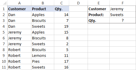
A usual VLOOKUP formula won't work in this situation because it returns the first found match based on a single lookup value that you specify.
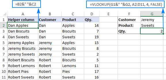
To overcome this, you can add a helper column and concatenate the values from two lookup columns (Customer and Product) there. It is important that the helper column should be the leftmost column in the table array because it's where Excel VLOOKUP always searches for the lookup value.
So, add a column to the left of your table and copy the below formula across that column. This will populate the helper column with the values from columns B and C (the space character is concatenated in between for better readability):
=B2&" "&C2
And then, use a standard VLOOKUP formula and place both criteria in the lookup_value argument, separated with a space:
=VLOOKUP("Jeremy Sweets", A2:D11, 4, FALSE)
Or, input the criteria in separate cells (G1 and G2 in our case) and concatenate those cells:
=VLOOKUP(G1&" "&G2, A2:D11, 4, FALSE)
As we want to return a value from column D, which is fourth in the table array, we use 4 for col_index_num. The range_lookup argument is set to FALSE to Vlookup an exact match. The screenshot below shows the result:
In case your lookup table is in another sheet, include the sheet's name in your VLOOKUP formula. For example:
=VLOOKUP(G1&" "&G2, Orders!A2:D11, 4, FALSE)
Alternatively, create a named range for the lookup table (say, Orders) to make the formula easier-to-read:
=VLOOKUP(G1&" "&G2, Orders, 4, FALSE)
For more information, please see How to Vlookup from another sheet in Excel.
Note. For the formula to work correctly, the values in the helper column should be concatenated exactly the same way as in the lookup_value argument. For example, we used a space character to separate the criteria in both the helper column (B2&" "&C2) and VLOOKUP formula (G1&" "&G2).
Formula 2. Excel VLOOKUP with multiple conditions
In theory, you can use the above approach to Vlookup more than two criteria. However, there are a couple of caveats. Firstly, a lookup value is limited to 255 characters, and secondly, the worksheet's design may not allow adding a helper column.
Luckily, Microsoft Excel often provides more than one way to do the same thing. To Vlookup multiple criteria, you can use either an INDEX MATCH combination or the XLOOKUP function recently introduced in Office 365.
For example, to look up based on 3 different values (Date, Customer name and Product), use one of the following formulas:
=INDEX(D2:D11, MATCH(1, (G1=A2:A11) * (G2=B2:B11) * (G3=C2:C11), 0))
=XLOOKUP(1, (G1=A2:A11) * (G2=B2:B11) * (G3=C2:C11), D2:D11)
Where:
- G1 is criteria 1 (date)
- G2 is criteria 2 (customer name)
- G3 is criteria 3 (product)
- A2:A11 is lookup range 1 (dates)
- B2:B11 is lookup range 2 (customer names)
- C2:C11 is lookup range 3 (products)
- D2:D11 is the return range (quantity)
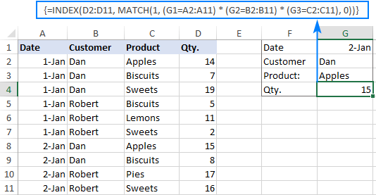
Note. In all versions except Excel 365, INDEX MATCH should be entered as an CSE array formula by pressing Ctrl + Shift + Enter. In Excel 365 that supports dynamic arrays it also works as a regular formula.
For the detailed explanation of the formulas, please see:
How to use VLOOKUP to get 2nd, 3rd or nth match
As you already know, Excel VLOOKUP can fetch only one matching value, more precisely, it returns the first found match. But what if there are several matches in your lookup array and you want to get the 2nd or 3rd instance? The task sounds quite intricate, but the solution does exist!
Formula 1. Vlookup Nth instance
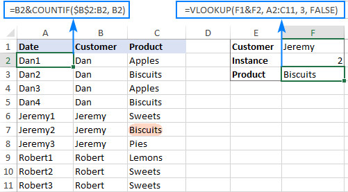
Suppose you have customer names in one column, the products they purchased in another, and you are looking to find the 2nd or 3rd product bought by a given customer.
The simplest way is to add a helper column to the left of the table like we did in the first example. But this time, we will populate it with customer names and occurrence numbers like "John Doe1", "John Doe2", etc.
To get the occurrence, use the COUNTIF function with a mixed range reference (the first reference is absolute and the second is relative like $B$2:B2). Since the relative reference changes based on a position of the cell where the formula is copied, in row 3 it will become $B$2:B3, in row 4 - $B$2:B4, and so on.
Concatenated with the customer name (B2), the formula takes this form:
=B2&COUNTIF($B$2:B2, B2)
The above formula goes to A2, and then you copy it down to as many cells as needed.
After that, input the target name and occurrence number in separate cells (F1 and F2), and use the below formula to Vlookup a specific occurrence:
=VLOOKUP(F1&F2, A2:C11, 3, FALSE)
Formula 2. Vlookup 2nd occurrence
If you are looking for the 2nd instance of the lookup value, then you can do without the helper column. Instead, create the table array dynamically by using the INDIRECT function together with MATCH:
=VLOOKUP(E1, INDIRECT("A"&(MATCH(E1, A2:A11, 0)+2)&":B11"), 2, FALSE)
Where:
- E1 is the lookup value
- A2:A11 is the lookup range
- B11 is the last (bottom-right) cell of the lookup table

Please note that the above formula is written for a specific case where data cells in the lookup table begin in row 2. If your table is somewhere in the middle of the sheet, use this universal formula, where A1 is the top-left cell of the lookup table containing a column header:
=VLOOKUP(E1, INDIRECT("A"&(MATCH(E1, A2:A11, 0)+1+ROW(A1))&":B11"), 2, FALSE)
How this formula works
Here is the key part of the formula that creates a dynamic vlookup range:
INDIRECT("A"&(MATCH(E1, A2:A11, 0)+2)&":B11")
The MATCH function configured for exact match (0 in the last argument) compares the target name (E1) against the list of names (A2:A11) and returns the position of the first found match, which is 3 in our case. This number is going to be used as the starting row coordinate for the vlookup range, so we add 2 to it (+1 to exclude the first instance and +1 to exclude row 1 with the column headers). Alternatively, you can use 1+ROW(A1) to calculate the necessary adjustment automatically based on the position of the header row (A1 in our case).
As the result, we get the following text string, which INDIRECT converts to a range reference:
INDIRECT("A"&5&":B11") -> A5:B11
This range goes to the table_array argument of VLOOKUP forcing it to start searching in row 5, leaving out the first instance of the lookup value:
VLOOKUP(E1, A5:B11, 2, FALSE)
How to Vlookup and return multiple values in Excel
The Excel VLOOKUP function is designed to return just one match. Is there a way to Vlookup multiple instances? Yes, there is, though not an easy one. This requires a combined use of several functions such as INDEX, SMALL and ROW is an array formula.
For example, the below can find all occurrences of the lookup value F2 in the lookup range B2:B16 and return multiple matches from column C:
{=IFERROR(INDEX($C$2:$C$11, SMALL(IF($F$1=$B$2:$B$11, ROW($C$2:$C$11)-1,""), ROW()-1)),"")}
There are 2 ways to enter the formula in your worksheet:
- Type the formula in the first cell, press Ctrl + Shift + Enter, and then drag it down to a few more cells.
- Select several adjacent cells in a single column (F1:F11 in the screenshot below), type the formula and press Ctrl + Shift + Enter to complete it.
Either way, the number of cells in which you enter the formula should be equal to or larger than the maximum number of possible matches.
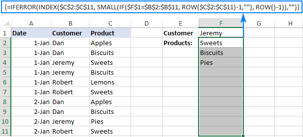
For the detailed explanation of the formula logic and more examples, please see How to VLOOKUP multiple values in Excel.
How to Vlookup in rows and columns (two-way lookup)
Two-way lookup (aka matrix lookup or 2-dimentional lookup) is a fancy word for looking up a value at the intersection of a certain row and column. There are a few different ways to do two-dimensional lookup in Excel, but since the focus of this tutorial is on the VLOOKUP function, we will naturally use it.
For this example, we'll take the below table with monthly sales and work out a VLOOKUP formula to retrieve the sales figure for a specific item in a given month.
With item names in A2:A9, month names in B1:F1, the target item in I1 and the target month in I2, the formula goes as follows:
=VLOOKUP(I1, A2:F9, MATCH(I2, A1:F1, 0), FALSE)

How this formula works
The core of the formula is the standard VLOOKUP function that searches for an exact match to the lookup value in I1. But since we do not know in which exactly column the sales for a specific month are, we cannot supply the column number directly to the col_index_num argument. To find that column, we use the following MATCH function:
MATCH(I2, A1:F1, 0)
Translated into English, the formula says: look up the I2 value in A1:F1 and return its relative position in the array. By supplying 0 to the 3rd argument, you instruct MATCH to find the value exactly equal to the lookup value (it's like using FALSE for the range_lookup argument of VLOOKUP).
Since Mar is in the 4th column in the lookup array, the MATCH function returns 4, which goes directly to the col_index_num argument of VLOOKUP:
VLOOKUP(I1, A2:F9, 4, FALSE)
Please pay attention that although the month names start in column B, we use A1:I1 for the lookup array. This is done in order for the number returned by MATCH to correspond to the column's position in table_array of VLOOKUP.
To learn more ways to perform matrix lookup in Excel, please see INDEX MATCH MATCH and other formulas for 2-dimensional lookup.
How to do multiple Vlookup in Excel (nested Vlookup)
Sometimes it may happen that your main table and lookup table do not have a single column in common, which prevents you from doing a Vlookup between two tables. However, there exists another table, which does not contain the information you are looking for but has one common column with the main table and another common column with the lookup table.
In below image illustrates the situation:
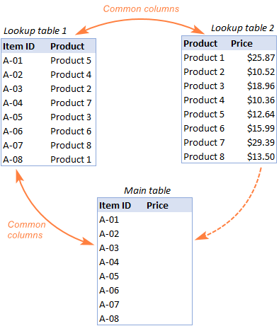
The goal is to copy prices to the main table based on Item IDs. The problem is that the table containing prices does not have the Item IDs, meaning we will have to do two Vlookups in one formula.
For the sake of convenience, let's create a couple of named ranges first:
- Lookup table 1 is named Products (D3:E10)
- Lookup table 2 is named Prices (G3:H10)
The tables can be in the same or different worksheets.
And now, we will perform the so-called double Vlookup, aka nested Vlookup.
First, make a VLOOKUP formula to find the product name in the Lookup table 1 (named Products) based on the item id (A3):
=VLOOKUP(A3, Products, 2, FALSE)
Next, put the above formula in the lookup_value argument of another VLOOKUP function to pull prices from Lookup table 2 (named Prices) based on the product name returned by the nested VLOOKUP:
=VLOOKUP(VLOOKUP(A3, Products, 2, FALSE), Prices, 2, FALSE)
The screenshot below shows our nested Vlookup formula in action:

How to Vlookup multiple sheets dynamically
Sometimes, you may have data in the same format split over several worksheets. And your aim is to pull data from a specific sheet depending on the key value in a given cell.
This may be easier to understand from an example. Let's say, you have a few regional sales reports in the same format, and you are looking to get the sales figures for a specific product in certain regions:

Like in the previous example, we start with defining a few names:
- Range A2:B5 in CA sheet is named CA_Sales.
- Range A2:B5 in FL sheet is named FL_Sales.
- Range A2:B5 in KS sheet is named KS_Sales.
As you can see, all the named ranges have a common part (Sales) and unique parts (CA, FL, KS). Please be sure to name your ranges in a similar manner as it's essential for the formula we are going to build.
Formula 1. INDIRECT VLOOKUP to dynamically pull data from different sheets
If your task is to retrieve data from multiple sheets, a VLOOKUP INDIRECT formula is the best solution – compact and easy-to-understand.
For this example, we organize the summary table in this way:
- Input the products of interest in A2 and A3. Those are our lookup values.
- Enter the unique parts of the named ranges in B1, C1 and D1.
And now, we concatenate the cell containing the unique part (B1) with the common part ("_Sales"), and feed the resulting string to INDIRECT:
INDIRECT(B$1&"_Sales")
The INDIRECT function transforms the string into a name that Excel can understand, and you put it in the table_array argument of VLOOKUP:
=VLOOKUP($A2, INDIRECT(B$1&"_Sales"), 2, FALSE)
The above formula goes to B2, and then you copy it down and to the right.
Please pay attention that, in the lookup value ($A2), we've locked the column coordinate with absolute cell reference so that the column remains fixed when the formula is copied to the right. In the B$1 reference, we locked the row because we want the column coordinate to change and supply an appropriate name part to INDIRECT depending on the column into which the formula is copied:

If your main table is organized differently, the lookup values in a row and unique parts of the range names in a column, then you should lock the row coordinate in the lookup value (B$1) and the column coordinate in the name parts ($A2):
=VLOOKUP(B$1, INDIRECT($A2&"_Sales"), 2, FALSE)

Formula 2. VLOOKUP and nested IFs to look up multiple sheets
In situation when you have just two or three lookup sheets, you can use a fairly simple VLOOKUP formula with nested IF functions to select the correct sheet based on the key value in a particular cell:
=VLOOKUP($A2, IF(B$1="CA", CA_Sales, IF(B$1="FL", FL_Sales, IF(B$1="KS", KS_Sales,""))), 2, FALSE)
Where $A2 is the lookup value (item name) and B$1 is the key value (state):

In this case, you do not necessarily need to define names and can use external references to refer to another sheet or workbook.
For more formula examples, please see How to VLOOKUP across multiple sheets in Excel.
That's how to use VLOOKUP in Excel. I thank you for reading and hope to see you on our blog next week!
Practice workbook for download
Advanced VLOOKUP formula examples (.xlsx file)
 by
by
540 comments
Hello,
I'm trying to make a meal plan tracker and I'm having a difficult time adding a formula to it.
One whole sheet is a food list with name, amount, calories, carbs, and fats. The other sheet is where I'm putting the formula and the columns are food, serving, calories, protein, carbs, fats.
I want to be able to input my food column and have it pull the info from the other sheet.
I was doing it column by column, this is what I have so far but it won't work:
=vlookup(vlookup(a2,list!$a$1:$f$41,0,false),calories,0,false)
pretty much I want to type in chicken and matches chicken from the other sheet, and pulls the values over. Thanks!
I am using the following formula as an array, but am getting blanks. Can you help resolve this please.
=IF(ISERROR(INDEX(Table_ExternalData_1[#All],SMALL(IF((Table_ExternalData_1[UserName]=$B$1)*(Table_ExternalData_1[comm_datetime]>=$B$2)*(Table_ExternalData_1[comm_datetime]=$B$2)*(Table_ExternalData_1[comm_datetime]<=$C$2),ROW(Table_ExternalData_1[UserName])),ROW(1:1)),4))
Basically trying to retrieve data using 3 criterias.
how to advance xxl
Maria,
I have sent in the excel file that I'm developing.
How to do two-way lookup in Excel??
in this you have showed how we could find second match result for the selected item only LEMON. which is very nice.
If suppose Same I need find for more than 20 items from the Raw data like more than 500 do I need to enter all 20 items individually or there is any short way for this.
Hi,
if i have below column or rows,
upc article no description
8901725121112 10108458 furnish ang
is it possible if i want description by upc and by article no in one cell.
Hi,
I have a Main table with many columns and rows. I have create a bill of matrials taking data from different columns. When I put a formula
=INDEX(B$4:$B$9,MATCH(F5,$A$4:$A$9,0),MATCH($G$3,$B$3:$D$3,0))/$B$10*$G$10
it also generate zero (0) values in rows data was not available.
My question is: I want to generate data with value in initial rows.
Kind regards,
Waseem
I have an excel spreadsheet that I'm attempt to do a vlookup or index to get detail of the monthly cost for cell phone to the first tab of a worksheet.
I have a tab for the details of multiple cell phones by month. it includes base costs, total minutes, text message, GB used, and so on.
I would like the front tab to pull the current month data from the detail sheet so the data can be reviewed monthly.
So I have created a tab that has the phone number, then a drop down menu for the month, then I need it to pull the data for that cell for that month.
This is where I get lost. I can get the data for the first instance but when you change the date nothing happens. I would appreciate any help you can provide.
Hello, Lance,
To help you better, we need a small sample table with your data in Excel. You can email it to support@ablebits.com. Please add the link to this article and your comment number.
Hi,
I'm currently looking for a function, that helps me sum up the numbers corresponding to the duplicate data in a different worksheet and this value to be brought to another sheet by vlookup.. In simple terms, a function that sums up and vlookup.
Parameters:
Name Start Date End Date Value
A 01-Apr-11 02-Feb-12 2
A 03-Feb-12 01-Mar-12 3
A 02-Mar-12 31-Dec-13 4
A 01-Jan-14 31-Jan-14 5
B 09-Jan-13 04-Apr-14 6
B 05-Apr-14 07-Feb-15 7
B 08-Feb-15 01-May-16 8
B 02-May-16 01-Jun-16 9
Name Date Value
A 30-Apr-12
A 05-Feb-12
A 30-Jan-14
B 07-Apr-14
B 20-Feb-15
Please help for for the above value column based on provided parameters.
Dear Sir,
I am doing vlookup in my time sheet there is four sheets i have done 1 sheet only balance 3 sheets i can't find please help me.
Dear Sir,
I Want to update leave code in attendence sheet according to leave trransaction on the basis of Employee code and respective dates from start date to end date remaining values in main sheet should be constant.
need your help on this. I want to vlook up for the specific number from another worksheet but the leftmost value is the combination of samenumber and some text I want the value in the 4th column. pls help
Hello, Loga,
To help you better, we need a sample table with your data in Excel. You can email it to support@ablebits.com. Please add the link to this article and your comment number.
great site......
could you help me with the below query.....
I am doing vlookup, my ref column will have duplicate but I need all their corresponding items in one single cell line by line... can u help me on this....
Hello Sudhakar,
Thank you for your feedback.
I'm sorry, but we don't know of a simple way to get all values in one cell. You may need to use VBA for this task.
You can get all values in different cells, please see the "Get all duplicate occurrences of the lookup value" section for a detailed description.
Then you can use the Concatenate function to merge all the values you get into one cell. Please see this post for more information:
https://www.ablebits.com/office-addins-blog/excel-concatenate-strings-cells-columns/
I have 4 columns of Reg. No. Name Subject and Grade. I want to return the grade of specific subject of a student how can I use the vlookup formula.
Hello Mubarak,
Please see the first part of this tutorial which describes examples of problems similar to yours:
https://www.ablebits.com/office-addins-blog/excel-vlookup-tutorial/
I love this Page.... I am a self learner and got lot of help from this page....
I have a large data for groups for e.g.
GRP_1 GRP_2 GRP_3
98465 5521 65466
65468 6663 6541
68465 6545 36541
65466 8466 6541
65466 9548 65666
and I want to create a list of products and which group it belongs like
Product Groups
5521 ??
6541 ??
6541 ?
6545
6663
8466
9548
36541
65466
65466
65466
65468
65666
68465
98465
Thanks
Hello, Ashwin,
Please try this formula:
=IF(ISERROR(MATCH(E2, $A$2:$A$6, 0)), IF(ISERROR(MATCH(E2, $B$2:$B$6, 0)), IF(ISERROR(MATCH(E2, $C$2:$C$6, 0)), "",$C$1), $B$1), $A$1)
Hey,
I loved you instructions! I have one question.
I am using INDEX MATCH to find a cell from another workbook and place the name of the cell near it. For example:
=INDEX('[Schedule 11.30.15 Hotschedules.xlsx]Sheet1'!$A$8:$A$75,MATCH($B$10,'[Schedule 11.30.15 Hotschedules.xlsx]Sheet1'!$C$8:$C$75,0))
Which works fine. But sometimes the "time" in the cell changes. For example $B$10 is "6:00 AM - 2:00 PM [Breads Sales]" but sometimes I use an employee that is only "6:00 AM - 1:30 PM [Breads Sales]". How can i make INDEX MATCH use 2 lookup values incase the first one fails?
Hello Argenis,
Try the IFERROR function that allows you to return another specified formula if the first one returns an error:
=IFERROR(INDEX('[Schedule 11.30.15 Hotschedules.xlsx]Sheet1'!$A$8:$A$75,MATCH(_$B$10_,'[Schedule 11.30.15 Hotschedules.xlsx]Sheet1'!$C$8:$C$75,0)),
INDEX('[Schedule 11.30.15 Hotschedules.xlsx]Sheet1'!$A$8:$A$75,MATCH(_$B$11_,'[Schedule 11.30.15 Hotschedules.xlsx]Sheet1'!$C$8:$C$75,0)))
https://support.office.com/en-us/article/IFERROR-function-c526fd07-caeb-47b8-8bb6-63f3e417f611
Thank you, It worked wonderfully!!!
Below was the table my scope of search
Customer Name Product
Brown Apples
HILL CHock
Brown Sweets
Acey Lollypop
Wolf chikky
Brown Biscuits
Hill Alapino
Wolf Jelly
Hill gems
Search Cell in the same Sheet like the following
$G2 $H2
Dan Brown Apples
Sweets
Biscuits
$G$5
Hill ????
????
?????
wolf
I had used the following formula to get the first set of search:
=IFERROR(INDEX($C$2:$C$16,SMALL(IF($G$2=$B$2:$B$16,ROW($C$2:$C$16)-1,""),ROW()-1)),"")
I like some help to expand (or) new formula to list all the duplicate values with respect to the string mention within the Left side, instead of hardcording the right side formula....that is $G$2
Thanks for looking and trying to help me out...!!!
Hello Pratap,
I recommend sorting the list and adding a column with the following formula:
=IF(COUNTIF($H$5:H5,H5)=1,CONCATENATE(H5," ",I5),I5)
Feel free to download a sample file that shows how it works:
https://support.ablebits.com/blog_samples/vlookup-formula-examples_102.xlsx
hello,
a have a question based on your example please:
if a have the next situation:
Dan Brown A B
Dan Brown C D
Jeremy Hill T I
Dan Brown R T
and I want to have the next result into another sheet :
Dan Brown A B C D R T
Jeremy Hill T I
How can I do that?
Hello Octav,
Please see our Combine Rows Wizard add-in:
https://www.ablebits.com/excel-combine-rows/index.php
In my opinion it help for your task if the values in columns A and B are merged into one.