The tutorial shows how to calculate trend in Excel by using the TREND function, how to create trends on a graph, and more.
These days when technologies, markets and customer needs are changing so rapidly, it is critical that you move with trends, and not against them. Trend analysis can help you identify underlying patterns in the past and current data movements and project future behavior.
Excel TREND function
The Excel TREND function is used to calculate a linear trend line through a given set of dependent y-values and, optionally, a set of independent x-values and return values along the trend line.
Additionally, the TREND function can extend the trendline into the future to project dependent y-values for a set of new x-values.
The syntax of the Excel TREND function is as follows:
Where:
Known_y's (required) - a set of the dependent y-values that you already know.
Known_x's (optional) - one or more sets of the independent x-values.
- If only one x variable is used, known_y's and known_x's can be ranges of any shape but equal dimension.
- If several x variables are used, known_y's must be a vector (one column or one row).
- If omitted, known_x's is assumed to be the array of serial numbers {1,2,3,...}.
New_x's (optional) - one or more sets of new x-values for which you want to calculate the trend.
- It must have the same number of columns or rows as known_x's.
- If omitted, it is assumed to be equal to known_x's.
Const (optional) - a logical value specifying how the constant a in the equation y = bx + a should be calculated.
- If TRUE or omitted, the constant a is calculated normally.
- If FALSE, the constant a is forced to 0, and the b-values are adjusted to fit the equation y = bx.
How TREND function calculates linear trendline
The Excel TREND Function finds the line that best fits your data by using the least squares method. The equation for the line is as follows.
For one range of x values:
y = bx + a
For multiple ranges of x values:
y = b1x1 + b2x2 + … + bnxn + a
Where:
- y - the dependent variable you are trying to calculate.
- x - the independent variable you are using to calculate y.
- a - the intercept (indicates where the line intersects the y-axis and is equal to the value of y when x is 0).
- b - the slope (indicates the steepness of the line).
This classic equation for the line of best fit is also used by the LINEST function and linear regression analysis.
TREND function as an array formula
To return multiple new y-values, the TREND function should be entered as an array formula. For this, select all the cells where you want the results to appear, type the formula and press Ctrl + Shift + Enter to complete it. As you do this, the formula will get enclosed in {curly braces}, which is a visual indication of an array formula. Since the new values are returned as an array, you won't be able to edit or delete them individually.
Excel TREND formula examples
At first sight, the syntax of the TREND function might seem excessively complicated, but the following examples will make things a lot easier.
TREND formula for time series trend analysis in Excel
Supposing you are analyzing some data for a sequential period of time and you want to spot a trend or pattern.
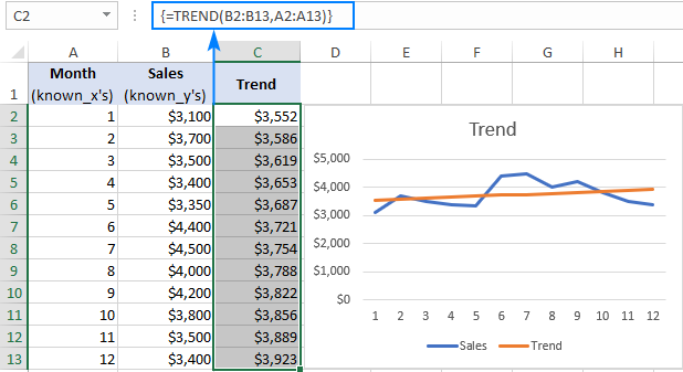
In this example, we have the month numbers (independent x-values) in A2:A13 and sales numbers (dependent y-values) in B2:B13. Based on this data, we want to determine the overall trend in the time series ignoring hills and valleys.
To have it done, select the range C2:C13, type the below formula and press Ctrl + Shift + Enter to complete it:
=TREND(B2:B13,A2:A13)
To draw the trendline, select the sales and trend values (B1:C13) and make a line chart (Insert tab > Charts group > Line or Area Chart).
As the result, you have both the numeric values for the line of best fit returned by the formula and a visual representation of those values in a graph:
Projecting a future trend
To predict a trend for the future, you just need to include a set of new x-values in your TREND formula.
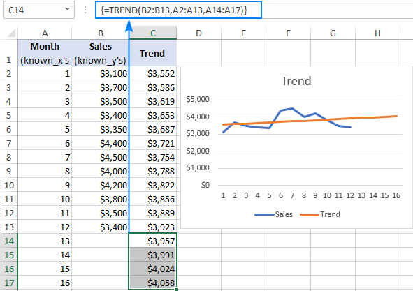
For this, we extend our time series with a few more month numbers and do trend projection by using this formula:
=TREND(B2:B13,A2:A13,A14:A17)
Where:
- B2:B13 is known_y's
- A2:A13 is known_x's
- A14:A17 is new_x's
Enter the above formula in cells C14:C17 and remember to press Ctrl + Shift + Enter to complete it appropriately. After that, create a new line chart for the extended data set (B1:C17).
The below screenshot shows the calculated new y-values and extended trendline:
Excel Trend formula for multiple sets of x-values
In situation when you have two or more sets of independent x values, enter them in separate columns, and supply that entire range to the known_x's argument of the TREND fucntion.
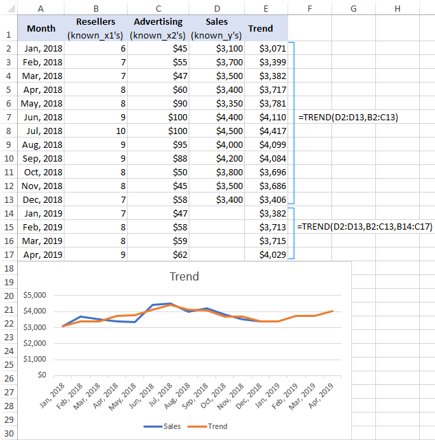
For example, with the known_x1 values in B2:B13, known_x2 values in C2:C13, and known_y values in D2:D13, you use the following formula to calculate trend:
=TREND(D2:D13,B2:C13)
Additionally, you can enter the new_x1 and new_x2 values in B14:B17 and C14:C17, respectively, and get the projected y-values with this formula:
=TREND(D2:D13,B2:C13,B14:C17)
If entered correctly (with the Ctrl + Shift + Enter shortcut), the formulas output the following results:
Other ways to do trend analysis in Excel
The TREND function is the most popular but not the only trend projection method in Excel. Below I will briefly describe a few other techniques.
Excel FORECAST vs TREND
"Trend" and "forecast" are very close concepts, but still there is a difference:
- Trend is something that represents the current or past days. For example, by analyzing the recent sales numbers, you can determine the cash flow trend and understand how your business has performed and is currently performing.
- Forecast is something that relates to the future. For example, by analyzing the historical data, you can project future changes and predict where current business practices will take you.
In terms of Excel, this distinction is not so obvious because the TREND function can not only calculate current trends, but also return future y-values, i.e. do trend forecasting.
The difference between TREND and FORECAST in Excel is as follows:
- The FORECAST function can only predict future values based on the existing values. The TREND function can calculate both current and future trends.
- The FORECAST function is used as a regular formula and returns a single new y-value for a single new-x value. The TREND function is used as an array formula and computes multiple y-values for multiple x-values.
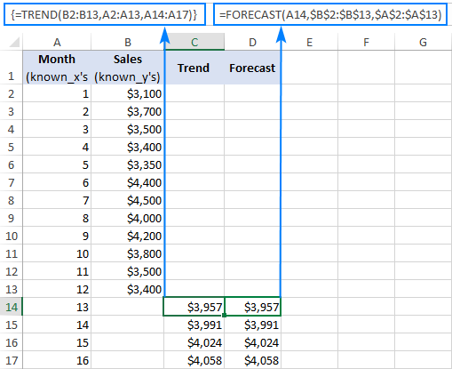
When used for time series forecasting, both functions produce the same linear trend/forecast because their calculations are based on the same equation.
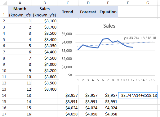
Please take a look at the screenshot below and compare the results returned by the following formulas:
=TREND(B2:B13,A2:A13,A14:A17)
=FORECAST(A14,$B$2:$B$13,$A$2:$A$13)
For more information, please see Using the FORECAST function in Excel.
Draw a trendline to visualize the trend
A trendline is commonly used to observe the general trend in your current data as well as project future data movements.
To add a trend to an existing chart, right-click the data series, and then click Add Trendline… This will create the default linear trendline for the current data and open the Format Trendline pane where you can choose another trendline type.
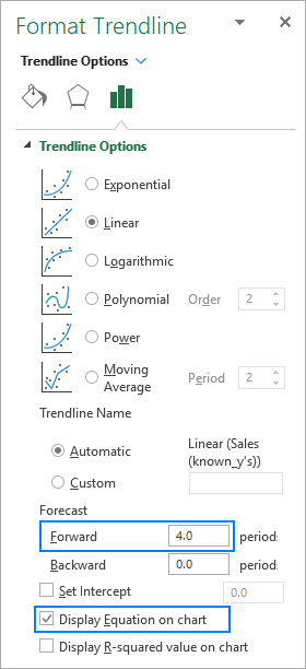
To forecast a trend, specify the number of periods under Forecast on the Format Trendline pane:
- To project the trend into the future, type the number of periods in the Forward box.
- To extrapolate a trend into the past, type the desired number in the Backward box.
To show the trendline equation, check the Display Equation on chart box. For better accuracy, you can show more digits in the trendline equation.
As shown in the image below, the results of the trendline equation are perfectly in line with the numbers returned by the FORECAST and TREND formulas:
For more information, please see How to add a trendline in Excel.
Smooth trend with moving average
Another simple technique that can help you show a trend is called moving average (aka rolling average or running average). This method smoothes out short-term fluctuations in a sample time series and highlights longer-term patterns or trends.
You can calculate moving average manually with your own formulas or have Excel make a trendline for you automatically.
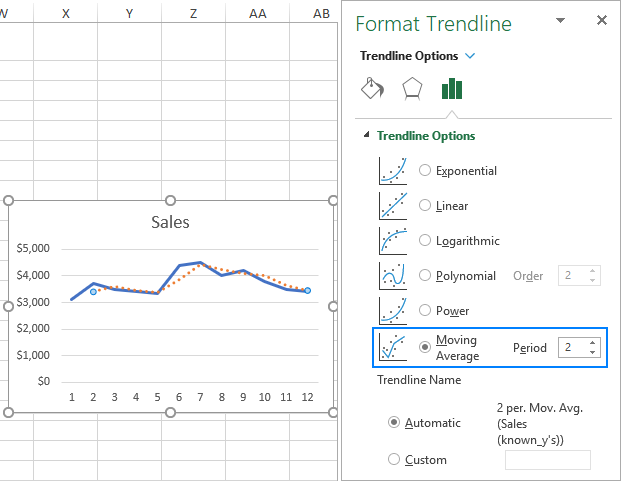
To display a moving average trendline on a chart, here's what you need to do:
- Right-click the data series and click Add Trendline.
- On the Format Trendline pane, select Moving Average and specify the desired number of periods.
That's how you use the TREND function to calculate trends in Excel. To have a closer look at the formulas discussed in this tutorial, you are welcome to download our sample Excel TREND workbook. I thank you for reading and hope to see you on our blog next week!
 by
by
14 comments
I've been trending my stock investment value for several years with both linear and exponential trend lines. with all returns reinvested. As this is essentially a compound savings investment, it is more closely modeled by the exponential trend equation. I'd like to differentiate the equation to determine the current rate of return. Unfortunately, substituting a current date value for the exponential exponent (x) results in wildly inaccurate results. Then I realized that the displayed coefficient of x was rounded to 4 decimal places with a single digit in the 4th decimal place. By trial and error I was able to extend the accuracy to 7 decimal places (4 significant digits) and get accurate results for y given a value of x from the trend line. Is there any way to get more accuracy (at least 4 significant digits) in the displayed x coef. when it becomes extremely small? Manually doing this thru trial and error is quite time consuming!
@Jeff, have you tried right clicking on the trendline equation, then formatting as a number with as many decimals as you want?
Hi Svetlana,
I have query to know. When I find a trend line from scatter point, we also get an equation of it. People ask question: what method( such as OLS estimation or MLE estimation), is used to get such trend line? How the excell has been programmed?
Prafulla
Hi Prafulla,
I am not an expert in this area, but I believe Excel uses OLS, assuming Ordinary Least Squares regression is another name for linear regression.
hello,
If anybody knows, please tell me how to add a bi-linear trend line in excel. help would be appreciated.
Hi!
You may find a couple of ideas in this excelforum.com thread.
Hello Dears,
Anybody can help with this issue please:
When I do trend, sometimes excel automatically consider empty cells as value 0 so the last line is declining slope in the excel till reach value of 0, how to stop this and make the last line in the trend is that showing a value as these empty cells supposed to be filled monthly (so it will be figure later on)
replace the 0 by #N/A and the cell content will be ingnored by the function. (it also works for graph display)
Is there any way to extract the coefficents of different independent variables ?
yes
Hello,
It seems that TREND function only works with a continuous range (set of cells), if we use a multiple selection of cells, for instance in your example above from lines 2 to 5 and 7 to 12, skipping line 6 both for known_y's and known_x's.
Is there a way to work with multiple selections, like it can be done with SUM function ?
Thanks in advance for your reply,
Infor
Hello Infor,
To my best knowledge, it is impossible. The syntax of the TREND function only provides for one known_y's and one known_x's range.
Hi Madam,
Request you can you share excel file with Trend & Forecasting Formula using.
Thanks & Regards,
Rakesh
Hi Rakesh,
Here is our sample workbook to using Trend and Forecasting functions in Excel:
Excel TREND function - sample workbook