In the previous blog post we successfully solved the problem of Excel not printing gridlines. Today I'd like to dwell on another issue related to Excel grid lines. In this article you'll learn how to show gridlines in an entire worksheet or in certain cells only, and how to hide lines by changing cells background or borders' color.
When you open an Excel document, you can see the horizontal and vertical faint lines that divide the worksheet into cells. These lines are called gridlines. It is very convenient to show gridlines in Excel spreadsheets as the key idea of the application is to organize the data in rows and columns. And you don't need to draw cell borders to make your data-table more readable.
All Excel spreadsheets have gridlines by default, but sometimes you can receive a sheet without cell lines from another person. In this case you may want them to become visible again. Removing lines is also a very common task. If you think that your spreadsheet will look more accurate and presentable without them, you can make Excel hide gridlines.
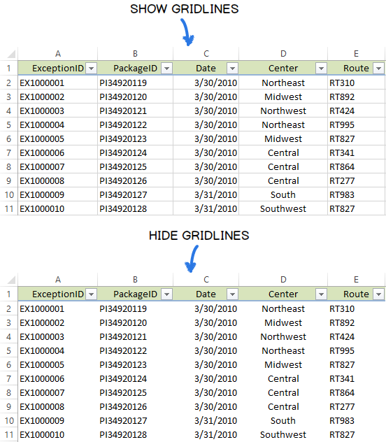
Whether you decide to show gridlines in your worksheet or hide them, go ahead and find below different ways to fulfil these tasks in Excel 2016, 2013 and 2010.
Show gridlines in Excel
Suppose you want to see gridlines in the entire worksheet or workbook, but they are just turned off. In this case you need to check one of the following options in the Excel 2016 - 2010 Ribbon.
Start with opening the worksheet where cell lines are invisible.
Note: If you'd like to make Excel show gridlines in two or more sheets, hold down the Ctrl key and click the necessary sheet tabs at the bottom of the Excel window. Now any changes will be applied to every selected worksheet.
When you are done with the selection, just navigate to the VIEW tab on the Ribbon and check the Gridlines box in the Show group.

Alternatively, you can go to the Sheet Options group on the PAGE LAYOUT tab and select the View checkbox under Gridlines.

Whichever option you choose gridlines will instantly appear in all the selected worksheets.
Note: If you want to hide gridlines in the entire spreadsheet, just uncheck the Gridlines or View options.
Show / hide gridlines in Excel by changing the fill color
One more way to display / remove gridlines in your spreadsheet is to use the Fill Color feature. Excel will hide gridlines if the background is white. If the cells have no fill, gridlines will be visible. You can apply this method for an entire worksheet as well as for a specific range. Let's see how it works.
- Select the necessary range or the entire spreadsheet.
Tip: The easiest way to highlight the whole worksheet is to click on the Select All button in the top-left corner of the sheet.
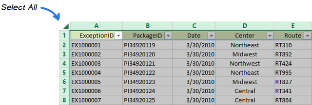
You can also use the Ctrl + A keyboard shortcut to select all the cells in the spreadsheet. You'll need to press the key combination twice or three times if your data is organized as Table.
- Go to the Font group on the HOME tab and open the Fill Color drop-down list.
- Choose the white color from the list to remove gridlines.
Note: If you want to show lines in Excel, pick the No Fill option.
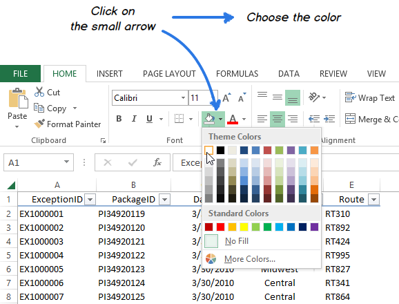
As you can see in the screenshot above, applying the white background will give an effect of hidden gridlines in your worksheet.
Make Excel hide gridlines only in specific cells
In case you want Excel to hide gridlines only in a certain block of cells, you can use the white cells background or apply white borders. Since you already know how to change the background color, let me show you how to remove gridlines by coloring the borders.
- Select the range where you want to remove lines.
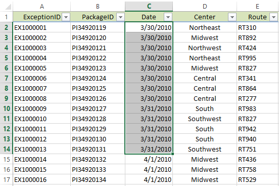
- Right-click on the selection and choose Format Cells from the context menu.
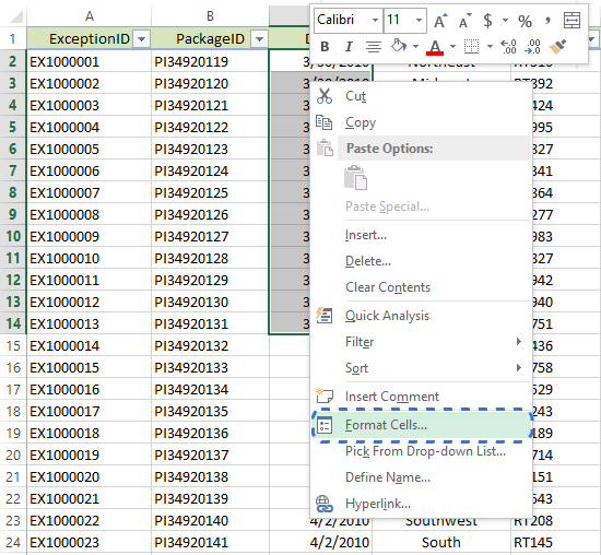
Note: You can also use the Ctrl + 1 keyboard shortcut to display the Format Cells dialog.
- Make sure that you are on the Border tab in the Format Cells window.
- Choose the white color and press the Outline and Inside buttons under Presets.
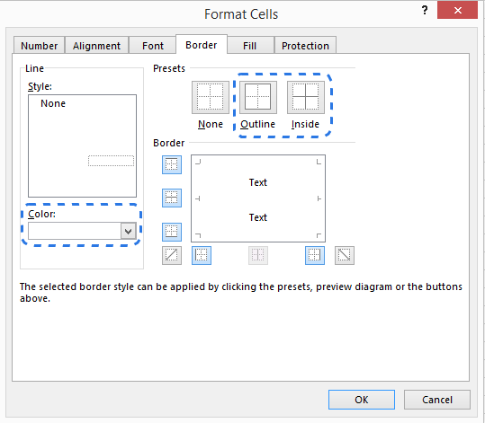
- Click OK to see the changes.
Here you go. Now you have an eye-catching "white crow" in your worksheet.
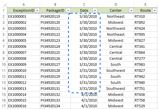
Note: To bring gridlines back to the block of cells, choose Noneunder Presets in the Format Cells dialog window.
Remove gridlines by changing their color
There is one more way to make Excel hide gridlines. If you change the default gridline color into white, gridlines will disappear in the whole worksheet. If you're interested in this method, feel free to find out how to change the default gridline color in Excel.
You see there are different ways to show and hide gridlines in Excel. Just choose the one that will work best for you. If you know any other methods of showing and removing cell lines, you are welcome to share them with me and other users! :)
 by
by
10 comments
I only want to copy the number inside a certain cell to the other cell having different border format. The problem is, the border were also copied. How am I suppose to do?
Hello Manny!
If you use the key shortcuts CRTL+C / CRTL+V or the Copy / Paste options from the context menu, you copy not only formulas or values, but the format of the cells as well. If you want to copy just values, please use the Paste Special option from the context menu or the CRTL+ALT+V key shortcut. In the dialog window opened please choose what exactly you want to insert into a cell.
None of these suggestions worked for me, I ended up figuring it out myself ... after wayyyy too long:
Go to the Home tab
Go to the Font section
Select the little square table icon
Select All Borders
Gridlines have returned!
I have maybe three strands of hair left after pulling out the rest.
Hope this helps someone.
Almost... the lines are back, but they aren't the same color as the default; now they're darker. There should be a button that says, "don't EVER mess with the grids." I can't be the only one.
Thank you!!!!! Seriously. SOOOOO MUCH!!! :)
Thanks Fluke! Came here years after, and nothing worked, but that worked. It's not perfect, but I'll take it.
Sometimes you find a set of three cells (arranged vertically) plus one more to the right of the middle one of the three, with no gridlines showing between them. In this case it seems (sometimes) that that middle one has been formatted unexpectedly. To cure, go to Format Cells, select the Fill tab, and click on No Colour (because even if you can't really see it, it turns out that the White button has been selected. This cured a puzzle for us!
This is the answer I've been searching for. Thank you!
This is what I use because I want colors but still wanted the faint gridline to organize the data.
My solution: Highlight the area you want the gridlines (likely the area you colored and lost them) - Right click - format cells - select the normal border size on the bottom left of the style box - under the color option select "Tan, Background 2" (this is a pre-set option third over right on the top selection - next ensure you select the type of border you want (this is the sample box that says "none, outline, inside, etc.) - finally click okay. You should now have a faint grid border that blends with the original grid marks un-noticingly (yes I made that word up :)
You can then use the same steps to add a black border around your new grid like border to better present your colored grid lined chart. :)
Thank you!!! I couldn't find this anywhere.