The tutorial explains the specificities of the Excel Rank functions and shows how to do ranking in Excel based on multiple criteria, rank data by group, calculate percentile rank, and more.
When you need to determine the relative position of a number in a list of numbers, the easiest way is to sort the numbers in ascending or descending order. If for some reason sorting is not possible, a Rank formula in Excel is the perfect tool to do the job.
Excel RANK function
The RANK function in Excel returns the order (or rank) of a numeric value compared to other values in the same list. In other words, it tells you which value is the highest, the second highest, etc.
In a sorted list, the rank of a certain number would be its position. The RANK function in Excel can determine the rank starting with the largest value (as if sorted in descending order) or the smallest value (as if sorted in ascending order).
The syntax of the Excel RANK function is as follows:
Where:
Number (required) - the value whose rank you'd like to find.
Ref (required) - a list of numeric values to rank against. It can be supplied as an array of numbers or a reference to the list of numbers.
Order (optional) - a number that specifies how to rank values:
- If 0 or omitted, the values are ranked in descending order, i.e. from largest to smallest.
- If 1 or any other non-zero value, the values are ranked in ascending order, i.e. from smallest to largest.
Excel RANK.EQ function
RANK.EQ is an improved version of the RANK function, introduced in Excel 2010. It has the same syntax as RANK and works with the same logic: if several values are ranked equally, the highest rank is assigned to all such values. (EQ stands for "equal").
In Excel 2007 and lower versions, you should always use the RANK function. In Excel 2010, Excel 2013, and Excel 2016, you can go with either RANK or RANK.EQ. However, it'd be wise to use RANK.EQ because RANK can be discontinued at any moment.
Excel RANK.AVG function
RANK.AVG is another function to find rank in Excel that is available only in Excel 2010, Excel 2013, Excel 2016 and later.
It has the same syntax as the other two functions:
The difference is that if more than one number has the same rank, the average rank is returned (AVG stands for "average").
4 things you should know about RANK in Excel
- Any Rank formula in Excel works only for numeric values: positive and negative numbers, zeros, date and time values. Non-numeric values in the ref argument are ignored.
- All RANK functions return the same rank for duplicate values, and skip subsequent ranking, as shown in the example below.
- In Excel 2010 and later versions, the RANK function has been replaced with RANK.EQ and RANK.AVG. For backward compatibility, RANK still works in all versions of Excel, but it may not be available in the future.
- If number is not found within ref, any Excel Rank function would return the #N/A error.
Basic Excel Rank formula (from highest to lowest)
To gain more understanding about ranking data in Excel, please have a look at this screenshot:

All three formulas rank numbers in column B in descending order (the order argument omitted):
In all versions of Excel 2003 - 2016:
=RANK($B2,$B$2:$B$7)
In Excel 2010 - 2016:
=RANK.EQ($B2,$B$2:$B$7)
=RANK.AVG($B2,$B$2:$B$7)
The difference is in how these formulas process duplicate values. As you see, the same score appears twice, in cells B5 and B6, which affects subsequent ranking:
- The RANK and RANK.EQ formulas give a rank of 2 to both duplicate scores. The next highest score (Daniela) is ranked 4th. A rank of 3 is not given to anyone.
- The RANK.AVG formula assigns a different rank to each duplicate behind the scenes (2 and 3 in this example), and returns the average of those ranks (2.5). Again, the 3rd rank is not assigned to anyone.
How to use RANK in Excel - formula examples
The path to excellence, they say, is paved with practice. So, to better learn how to use RANK function in Excel, alone or in combination with other functions, let's work out solutions to a few real-life tasks.
How to rank in Excel from lowest to highest
As shown in the above example, to rank numbers from highest to lowest, you use one of the Excel Rank formulas with the order argument set to 0 or omitted (default).
To have number ranked against other numbers sorted in ascending order, put 1 or any other non-zero value in the optional third argument.
For example, to rank the 100-meter sprint times of the students, you can use either of the below formulas:
=RANK(B2,$B$2:$B$7,1)
=RANK.EQ(B2,$B$2:$B$7,1)
Please pay attention that we lock the range in the ref argument by using absolute cell references, so that it won't change when we copy the formula down the column.
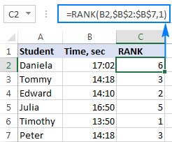
As the result, the lowest value (fastest time) is ranked 1st and the largest value (slowest time) gets the lowest rank of 6. The equal times (B2 and B7) are given the same rank.
How to rank data in Excel uniquely
As pointed out earlier, all of the Excel Rank functions return the same rank for items of equal value. If that's not want you want, use one of the following formulas to resolve tie-break situations and give a unique rank to each number.
Unique ranking from highest to lowest
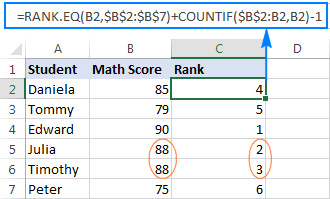
To rank the math scores of our students uniquely in descending order, use this formula:
=RANK.EQ(B2,$B$2:$B$7)+COUNTIF($B$2:B2,B2)-1
Unique ranking from lowest to highest
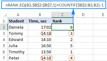
To rank the 100-meter race results in ascending order with no duplicates, use this formula:
=RANK.EQ(B2,$B$2:$B$7,1) + COUNTIF($B$2:B2,B2)-1
How these formulas work
As you may have noticed, the only difference between the two formulas is the order argument of the RANK.EQ function: omitted to rank values descending, 1 to rank ascending.
In both formulas, it's the COUNTIF function with the clever use of relative and absolute cell references that does the trick. In short, you use COUNTIF to find out how many occurrences of the number being ranked there are in the above cells, including the number's cell. In the topmost row where you enter the formula, the range consists of a single cell ($B$2:B2). But because you lock only the first reference ($B$2), the last relative reference (B2) changes based on the row where the formula is copied. Thus, for row 7, the range expands to $B$2:B7, and the value in B7 is compared to each of the above cells.
Consequently, for all 1st occurrences, COUNTIF returns 1; and you subtract 1 at the end of the formula to restore the original rank.
For 2nd occurrences, COUNTIF returns 2. By subtracting 1 you increment the rank by 1 point, thus preventing duplicates. If there happen to be 3 occurrences of the same value, COUNTIF()-1 would add 2 to their ranking, and so on.
Alternative solution to break Excel RANK ties
Another way to rank numbers in Excel uniquely is by adding up two COUNTIF functions:
- The first function determines how many values are greater than or less than the number to be ranked, depending on whether you are ranking descending or ascending, respectively.
- The second function (with the "expanding range" $B$2:B2 as in the above example) gets the number of values equal to the number.
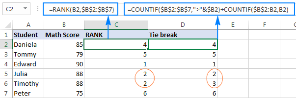
For example, to rank numbers uniquely from highest to lowest, you'd use this formula:
=COUNTIF($B$2:$B$7,">"&$B2)+COUNTIF($B$2:B2,B2)
As shown in the screenshot below, the tie-break is successfully resolved, and a unique rank is assigned to each student:
Ranking in Excel based on multiple criteria
The previous example has demonstrated two working solutions for an Excel RANK tie break situation. However, it may seem unfair that equal numbers are ranked differently based solely on their position in the list. To improve your ranking, you may want to add one more criteria to be considered in case of a tie.
In our sample dataset, let's add total scores in column C and calculate rank as follows:
- First, rank with Math Score (main criteria)
- When there is a tie, break it with Total Score (secondary criteria)
To have it done, we will be using a regular RANK/RANK.EQ formula to find rank, and the COUNTIFS function to break a tie:
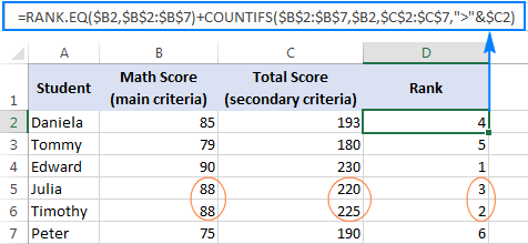
=RANK.EQ($B2,$B$2:$B$7) + COUNTIFS($B$2:$B$7, $B2, $C$2:$C$7, ">"& $C2)
Compared to the above example, this rank formula is more objective: Timothy is ranked 2nd because his total score is higher than that of Julia:
How this formula works
The RANK part of the formula is obvious, and the COUNTIFS function does the following:
- The first criteria_range/criteria pair ($B$2:$B$7,$B2) counts the occurrences of the value you are ranking. Please notice, we fix the range with absolute references, but do not lock the criteria's row ($B2) so that the formula checks the value in each row individually.
- The second criteria_range/criteria pair ($C$2:$C$7,">"&$C2) finds out how many total scores are greater than the total score of the value being ranked.
Because COUNTIFS works with the AND logic, i.e. counts only cells that meet all of the specified conditions, it returns 0 for Timothy since no other student with the same Math score has a higher total score. Hence, Timothy's rank returned by RANK.EQ is unchanged. For Julia, the COUNTIFS function returns 1 because one student with the same Math score has a higher total, so her rank number is incremented by 1. If one more student had the same Math score and a total score lower than that of Timothy and Julia, his/her rank would be incremented by 2, and so on.
Alternative solutions to rank numbers with multiple criteria
Instead of the RANK or RANK.EQ function, you could use COUNTIF to check the main criteria, and COUNTIFS or SUMPRODUCT to resolve a tie break:
=COUNTIF($B$2:$B$7,">"&$B2) + COUNTIFS($B$2:$B$7, $B2, $C$2:$C$7, ">"&$C2) + 1
=COUNTIF($B$2:$B$7, ">"&$B2) + SUMPRODUCT(--($B$2:$B$7=$B2), --($C$2:$C$7>$C2)) + 1
The result of these formulas are exactly the same as shown above.
How to calculate percentile rank in Excel
In statistics, a percentile (or centile) is the value below which a certain percentage of values in a given dataset falls. For example, if 70% of students are equal to or below your test score, your percentile rank is 70.
To get percentile rank in Excel, use the RANK or RANK.EQ function with a non-zero order argument to rank numbers from smallest to largest, and then divide the rank by the count of numbers. So, the generic Excel Percentile Rank formula goes as follows:
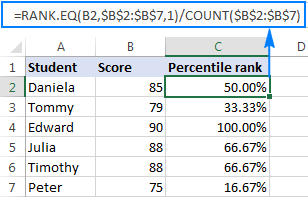
To calculate the percentile rank of our students, the formula takes the following shape:
=RANK.EQ(B2,$B$2:$B$7,1)/COUNT($B$2:$B$7)
To have the results displayed correctly, be sure to set the Percentage format to the formula cells:
How to rank numbers in non-adjacent cells
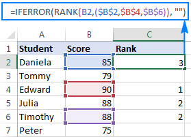
In situations when you need to rank non-contiguous cells, supply those cells directly in the ref argument of your Excel Rank formula in the form of a reference union, locking the references with the $ sign. For example:
=RANK(B2,($B$2,$B$4,$B$6))
To prevent errors in non-ranked cells, wrap RANK in the IFERROR function, like this:
=IFERROR(RANK(B2,($B$2,$B$4,$B$6)), "")
Please notice that a duplicate number is also given a rank, though cell B5 is not included in the formula:
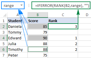
If you need to rank multiple non-contiguous cells, the above formula may become too long. In this case, a more elegant solution would be defining a named range, and referencing that name in the formula:
=IFERROR(RANK(B2,range), "")
How to rank in Excel by group
When working with entries organized into some kind of data structure, data may belong to various groups, and you might want to rank numbers within each group individually. The Excel RANK function cannot resolve this challenge, so we are going to use a more complex SUMPRODUCT formula:
Rank by group in descending order:
=SUMPRODUCT((A2=$A$2:$A$7)*(C2<$C$2:$C$7))+1
Rank by group in ascending order:
=SUMPRODUCT((A2=$A$2:$A$7)*(C2>$C$2:$C$7))+1
Where:
- A2:A7 are groups assigned to numbers.
- C2:C7 are numbers to be ranked.
In this example, we use the first formula to rank numbers in each group from largest to smallest:
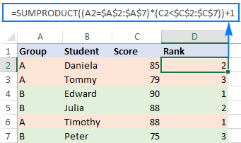
How this formula works
Essentially, the formula evaluates 2 conditions:
- First, you check the group (A2=$A$2:$A$7). This part returns an array of TRUE and FALSE based on whether a range element belongs to the same group as A2.
- Second, you check the score. To rank values from largest to smallest (descending order), use the condition (C2<$C$2:$C$11), which returns TRUE for the cells greater than or equal to C2, FALSE otherwise.
Since in Microsoft Excel terms, TRUE = 1 and FALSE = 0, multiplying the two arrays gives an array of 1's and 0's, where 1 is returned only for the rows in which both conditions are met.
Then, SUMPRODUCT adds up the elements of the 1's and 0's array, hence returning 0 for the largest number in each group. And you add 1 to the result to start ranking with 1.
The formula that ranks numbers within groups from smallest to largest (ascending order) works with the same logic. The difference is that SUMPRODUCT returns 0 for the smallest number in a particular group, since no number in that group meets the 2nd condition (C2>$C$2:$C$7). Again, you replace zero rank with the 1st rank by adding 1 to the formula result.
Instead of SUMPRODUCT, you can use the SUM function to add up the array elements. But this would require using an array formula, completed via Ctrl + Shift + Enter. For example:
=SUM((A2=$A$2:$A$7)*(C2<$C$2:$C$7))+1
How to rank positive and negative numbers separately
If your list of numbers contains both positive and negative values, the Excel RANK function will rank them all in no time. But what if you'd like to have positive and negative numbers ranked separately?
With numbers in cells A2 to A10, use one of the following formulas to get individual ranking for positive and negative values:
Rank positive numbers descending:
=IF($A2>0,COUNTIF($A$2:$A$10,">"&A2)+1,"")
Rank positive numbers ascending:
=IF($A2>0,COUNTIF($A$2:$A$10,">0")-COUNTIF($A$2:$A$10,">"&$A2),"")
Rank negative numbers descending:
=IF($A2<0,COUNTIF($A$2:$A$10,"<0")-COUNTIF($A$2:$A$10,"<"&$A2),"")
Rank negative numbers ascending:
=IF($A2<0,COUNTIF($A$2:$A$10,"<"&$A2)+1,"")
The results will look something similar to this:
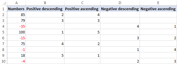
How these formulas work
To begin with, let's break down the formula that ranks positive numbers in descending order:
- In the logical test of the IF function, you check whether the number is greater than zero.
- If the number is greater than 0, the COUNTIF function returns the count of values higher than the number being ranked.
In this example, A2 contains the 2nd highest positive number, for which COUNTIF returns 1, meaning there is just one number greater than it. In order to start our ranking with 1, not 0, we add 1 to the formula result, so it returns a rank of 2 for A2.
- If the number is greater than 0, the formula returns an empty string ("").
The formula that ranks positive numbers in ascending order works a bit differently:
If the number is greater than 0, the first COUNTIF gets the total count of positive numbers in the data set, and the second COUNTIF finds out how many values are higher than that number. Then, you subtract the latter from the former, and get the desired rank. In this example, there are 5 positive values, 1 of which is greater than A2. So, you subtract 1 from 5, thus getting a rank of 4 for A2.
Formulas to rank negative numbers are based on a similar logic.
Note. All of the above formulas ignore zero values because 0 belongs neither to the set of positive nor to the set of negative numbers. To include zeros in your ranking, replace >0 and <0 with >=0 and <=0, respectively, where the formula logic requires.
For example, to rank positive numbers and zeros from largest to smallest, use this formula: =IF($A2>=0,COUNTIF($A$2:$A$10,">"&A2)+1,"")
How to rank data in Excel ignoring zero values
As you already know, a RANK formula is Excel handles all numbers: positive, negative and zeros. But in some cases, we just want to rank cells with data ignoring 0 values. On the web, you can find a few possible solutions for this task, but the Excel RANK IF formula, methinks, is the most universal one:
Rank numbers descending ignoring zero:
=IF($B2=0,"",IF($B2>0,RANK($B2,$B$2:$B$10), RANK($B2,$B$2:$B$10)-COUNTIF($B$2:$B$10,0)))
Rank numbers ascending ignoring zero:
=IF($B2=0,"",IF($B2>0,RANK($B2,$B$2:$B$10,1) - COUNTIF($B$2:$B$10,0), RANK($B2,$B$2:$B$10,1)))
Where B2:B10 is the range of numbers to be ranked.
The best thing about this formula is that it works beautifully both for positive and negative numbers, leaving zero values out of ranking:
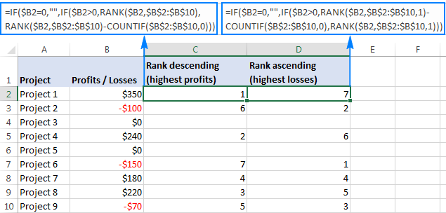
How this formula works
At first sight, the formula may seem a bit tricky. Upon a closer look, the logic is very simple.
Here's how the Excel RANK IF formula ranks numbers from largest to smallest ignoring zeros:
- The first IF checks whether the number is 0, and if it is, returns an empty string:
IF($B2=0,"", …)
- If the number is not zero, the second IF checks whether it's greater than 0, and if it is, a regular RANK / RANK.EQ function calculates its rank:
IF($B2>0,RANK($B2,$B$2:$B$10),…)
- If the number is less than 0, you adjust ranking by the zero count. In this example, there are 4 positive numbers and 2 zeros. So, for the largest negative number in B10, an Excel RANK formula would return 7. But we skip zeros, and therefore we need to adjust the rank by 2 points. For this, we subtract the number of zeros from the rank:
RANK($B2,$B$2:$B$10)-COUNTIF($B$2:$B$10,0))
Yep, it's that easy! The formula to ranks numbers from smallest to largest ignoring zeroes works in a similar manner, and it could be a good brain exercise to deduce its logic :)
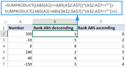
How to calculate rank in Excel by absolute value
When dealing with a list of positive and negative values, there may be a need to rank numbers by their absolute values ignoring the sign.
The task can be fulfilled with one of the bellow formulas, at the heart of which is the ABS function that returns the absolute value of a number:
Rank ABS descending:
=SUMPRODUCT((ABS(A2)<=ABS(A$2:A$7)) * (A$2:A$7<>"")) - SUMPRODUCT((ABS(A2)=ABS($A$2:$A$7)) * (A$2:A$7<>""))+1
Rank ABS ascending:
=SUMPRODUCT((ABS(A2)>=ABS(A$2:A$7)) * (A$2:A$7<>"")) - SUMPRODUCT((ABS(A2)=ABS($A$2:$A$7)) * (A$2:A$7<>""))+1
As the result, negative numbers are ranked as if they were positive numbers:
How to get N largest or smallest values
If you wish to get an actual N number of the largest or smallest values rather than their ranking, use the LARGE or SMALL function, respectively.
For example, we can get the top 3 scores of our students with this formula:
=LARGE($B$2:$B$7, $D3)
Where B2:B7 is the list of scores and D3 is the desired rank.
Additionally, you can retrieve the students' names by using the INDEX MATCH formula (provided there are no duplicate scores in the top 3):
=INDEX($A$2:$A$7,MATCH(E3,$B$2:$B$7,0))
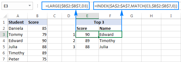
Similarly, you can use the SMALL function to pull the bottom 3 values:
=SMALL($B$2:$B$7, $D3)
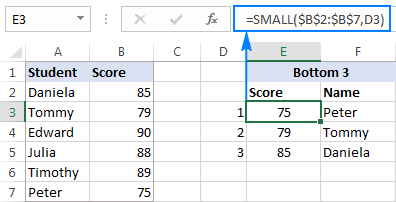
That's how you do ranking in Excel. I thank you for reading and hope to see you on our blog next week!
Practice workbook for download
Rank formula in Excel - examples (.xlsx file)
 by
by
153 comments
I have data for which I have calculated their mean, median, mode, standard deviation. how do I calculate their rank ? should I only use mean (highest mean would be rank 1 and so on ) or should I use ''mean divided by standard deviation, i.e. signal to noise ratio (snr) '' to calculate their rank in excel? please help!
this is the data that I need help with.
MEAN SD
4.4 0.753937035
4.45 0.944513241
4.05 1.145931017
4.75 0.550119604
4.5 0.827170192
4.35 0.74515982
4.45 0.887041208
4.05 0.944513241
Hi, I have a set of numbers:
0,0591
0,0556
0,1163
-5,7416
0,8221
-0,5554
1,0672
1,8117
0,8832
0
0,2268
1,2297
1,5574
0,6483
6,2281
2,4252
2,8033
5,7375
1,8332
0,7603
1,7136
0,2329
I need to rank them closest to 0, with 0 being ranked 1, that's an easy part. But I need to treat the negative numbers as being the last on the ranking order.
Thank You in advance!
Hello!
Sorry, I do not fully understand the task. What does the “I need to rank them closest to 0, with 0 being ranked 1” phrase mean? Give an example of the expected result.
Hi, sorry for the confusion. Here's my task:
List Rank Rank Needed
0,0556 4 2
0,1163 6 4
0,8221 11 9
0,0591 5 3
0,4831 9 7
-5,7416 1 14
1,0672 13 11
0,7626 10 8
1,8117 14 12
0,8832 12 10
0 3 1
0,3405 8 6
0,2268 7 5
-0,5554 2 13
I use this formula, to begin with, RANK(A2;$A$2:$A$15;1), to start the list with 0 i use this: IF(A2>=0;RANK(A2;$A$2:$A$15;1)-COUNTIF($A$2:$A$15;"<0")). My question is how do I add the negative numbers to the back of my ranking list?
Hello!
If I got you right, the formula below will help you with your task:
=IF(A1>=0,COUNTIF($A$1:$A$14,">=0") - COUNTIF($A$1:$A$14,">"&$A1), COUNTIF($A$1:$A$14,"<0") - COUNTIF($A$1:$A$14,"<"&$A1) + COUNTIF($A$1:$A$14,">=0"))
Pay attention to the following paragraph of the article above — Rank positive and negative numbers separately
Perfect! ?
I believe in the last message I sent you regarding Ranking on Every Nth Column my formula showed E2 for the search value, it should have been F2 since the formula is searching on every other other column (Modulus 2). The formula should have been as below. This still get the SPILL error. I'd greatly appreciate if you had a solution to this. Thanks.
=RANK.EQ(F2,IF(MOD(COLUMN($A2:$J2)-COLUMN($A2)+1,2)=0,$A2:$J2))
Hello!
#SPILL! is a new Excel error that only occurs when a dynamic array hasn't enough place to display the result. There should be enough blank cells around your formula for it to write the results of the calculations. If these cells are occupied by formulas or values, an error will occur.
For more information, please see Excel #SPILL! error - causes and fixes.
Hi Folks,
I use the Max of every nth Column using an approach from ExcelJet in the link below . When I try this with the RANK or RANK.EQ functions, I get a spill error. for example using the formula where the array of values in columns A2 though K2, and attempting to get the rank of cell E2 from every other column ( the ,2 in the formula)
=RANK(E2,IF(MOD(COLUMN($A2:$J2)-COLUMN($A2)+1,2)=0,$A2:$J2))
Is it possible to get the rank of a value from a range of numbers from every nth column?
Thank you.
Mike
https://exceljet.net/formula/max-of-every-nth-column#:~:text=To%20get%20the%20max%20of%20every%20nth%20column%2C,be%20entered%20with%20control%20%2B%20shift%20%2B%20enter.
Hi there to all followers of this...
With regards to the simple excel rank function.
Anyone have an idea on how to start the order from a particular given number as opposed to starting from 1?
i.e Manipulate the Order (optional) - a number that specifies how to rank values.
The only options with rank eq appear to be:
If 0 or omitted, the values are ranked in descending order, i.e. from largest to smallest.
If 1 or any other non-zero value, the values are ranked in ascending order, i.e. from smallest to largest.
Many Thanks,
Bobby.
Hello!
For me to be able to help you better, please specify which formula you mean and describe the problem in more detail. If you want to get the N largest values starting from 1, change the second parameter in the LARGE function. It's hard for me to guess from your description, but maybe this will help.
PLS help me with this: I would like to rank only those from 80 and above with 90 as the highest or rank 1.
80
75
83
88
79
90
thanks :-)
i got it this way! i just combined rank() with IF():
=if(A2>79,rank(A2,$A$2:$A$7),"")
thanks anyway :-)
Hi, my doubt is,how to get same rank holders names in a single cell?
Hello!
I’m sorry but your task is not entirely clear to me. For me to be able to help you better, please describe your task in more detail. Please specify what you were trying to find. Give an example of the source data and the expected result.
It’ll help me understand it better and find a solution for you.
Hey, I want to rank by group but I also have duplicate values, whats the best formula without it duplicating/skipping the rank?
Thanks!
duplicate and skipping the rank number I mean as below :)
Rank Style WEEKEND SALES
1 MZZ6495 556
2 MZZ2170 210
2 MZZ2282 210
2 MZZ1560 210
5 MZZ1539 203
6 MZZ2443 178
7 MZZ1982 151
Hello!
The article above describes how to rank with duplicates and without duplicates.
Please specify what you were trying to find, what formula you used and what problem or error occurred. Give an example of the source data and the expected result.
It’ll help me understand it better and find a solution for you. Thank you.
Hi,
i need to understand, how formula works and generates percentage number ranking?
Name Amount Percentage
majid 20 14.29%
sajid 70 85.71%
ahmed 80 100.00%
sultan 40 71.43%
khan 30 42.86%
majid 20 14.29%
sajid 35 57.14%
the formula i used =RANK.EQ(B2,$B$2:$B$8,1)/COUNT($B$2:$B$8)
first one Majid 20 percentage 14.29%. if i divide (20/7*100) is not correct. can you explain the break up of this formula, how works?
Thanks
Hi,
Fantastic. But what if i want to assign only 3 rank (1st, 2nd, 3rd)?
If the column for group is starting with a number like 2B, 2E 2C 2S then the ranks for some is +2 or +1 please help
Does any know how to fix the issue with Excel 2022 crashing on startup?
Hi Kevin, try this
=SUMPRODUCT((A1>=$A$1:$A$10)/COUNTIF($A$1:$A$10,$A$1:$A$10))
Y'all got some tips for ranking without skipping a number yo!
Hello!
I have 179. Is it possible to rank each subject such that student A will be like position 2/179 or 5/179 or 1/179?
I really need help. Please??? help me.
HI,I Want to calculate rank for students those who are passed in all subjects only,
if the passing mark is 7 out of 20.please help
How can I rank on test scores, where anybody scoring over 95% automatically top ranked (1 - ties are ok); and anybody scoring less than 95% is then ranked by total # of test scores?
Student - Score - Rank
Billy - 50% - Rank 5
Ralph - 45% - Rank 6
Shelly - 96% - Rank 1
Luis - 95% - Rank 1
Lucy - 97% - Rank 1
Shay - 94% - Rank 2
Monica - 70% - Rank 3
Sarah - 68% - Rank 4
Joe - 98% - Rank 1
Mel - 33% - Rank 10
EDIT:
Student - Score - Rank
Billy - 50% - Rank 8
Ralph - 45% - Rank 9
Shelly - 96% - Rank 1
Luis - 95% - Rank 1
Lucy - 97% - Rank 1
Shay - 94% - Rank 5
Monica - 70% - Rank 6
Sarah - 68% - Rank 7
Joe - 98% - Rank 1
Mel - 33% - Rank 10
Hello Juan,
Thank you for your comment. Here is the formula that should do the trick for you:
=IF(B2 < 95, COUNTIF($B$2:$B$11, " > "&B2)+COUNTIF($B$2:$B$11, " = "&B2), 1)
Funds 1M 3M 6M YTD 1Y
Fund1 3% 7% 12% 10% 17%
Fund2 3% 7% 12% 10% 17%
Fund3 7% 8% 9% 12% 6%
Fund4 -5% -11% 22% 14% 23%
Fund5 10% 16% 14% 15% 26%
Fund6 0% 3% 19% 19% 20%
Fund7 -1% 2% 19% 20% 19%
Fund8 -2% 2% 19% 20% 19%
Fund9 0% 3% 20% 20% 21%
Fund10 3% 7% 12% 10% 17%
Hi Olive, how can we rank data like this with excel formula to find which is the best performing...
How do you prevent the rank from repeating itself...like two values given 1...at the same time
Hi Olive,
Check out these solutions: How to rank numbers uniquely
How to rank this by excel formula?
Carrier POL POD Rate (Dollar) Rank
Carrier A PGU Jakarta 100 1
Carrier B PGU Jakarta 200 2
Carrier C PGU Jakarta 300 3
Carrier D PGU Jakarta 400 4
Carrier A PGU Rotterdam 500 4
Carrier B PGU Rotterdam 400 3
Carrier C PGU Rotterdam 300 2
Carrier D PGU Rotterdam 200 1
Carrier A SGP Jakarta 100 1
Carrier B SGP Jakarta 200 2
Carrier C SGP Jakarta 300 3
Carrier D SGP Jakarta 400 4
Carrier A SGP Rotterdam 500 4
Carrier B SGP Rotterdam 400 3
Carrier C SGP Rotterdam 300 2
Carrier D SGP Rotterdam 200 1
How ranking group on multiple criteria?
kindly help to prepare formula
problem of multi conditional ranking. Example. Students got 500,450,400,350,300,250 respectively,Number of their fail subjects r 0,0,1,1,2,2 respectively Their ranks should be as 1,2,3,4,5 ,6. Please help to prepare formula.
How to calculate the students merit so that the highest are on top and lowest in the decreasing order
Excellent! after trying various methods, RANK.EQ($B2,$B$2:$B$7)+COUNTIFS($B$2:$B$7,$B2,$C$2:$C$7,">"&$C2) really worked for ranking with 4 columns!
Thanks
I have 20 golfers with all their gross scores from holes 1 through 18 and a total gross ... all that data in a row for each golfer. We pay 4 best gross scores. When there is a tie we go back to each hole starting at hole #1 and look for the lower score(s) which eliminates the other golfers for this payout. Then go to next hole and continue until there is only 1 golfer remaining who gets this payout award for the rank position ($40 for 1st, $30 for 2nd, $20 for 3rd, $10 for 4th). We encountered a situation where 4 golfers had the same GROSS score, on hole #1 2 of them had the same score and better (lower) than the other 2. The tie between these lower 2 finally broke by hole #10; this determined payouts for 1st and 2nd. Of the remaining 2 golfers to determine payout 3 and 4, the tie break came on hole # 5. We did all this manually/visually. Can we get this in xls formulas?? Thank you.
btw ... tie breaks is a common occurrence in golf so a formula solution would help many tournament organizers.
yes, you can do this through code in excel
Help me how to rank multiple categories. First pass and fail. Second look at mark
Is there any way to do rank where you don't skip?
For instance
Score Rank
30 1
28 2
28 2
27 4
I would like it so that the 27 is a 3, is this possible?
I found an answer to this...
=SUMPRODUCT((G2 < G$2:G$27)/COUNTIF(G$2:G$27,G$2:G$27))+1
Is there any way to do the above based on a value in another column? Let's say column A contains a group number assignment (1,2 and 3).
Mathew Collen, what you are asking about is my current dilemma. Did you ever find an answer?
Hi all, I am trying to get a priority ranked list based on "Impact" (where highest number is higher impact) vs "Effort" (where lowest number is lowest effort), I want to basically get highest "Impact" / low "Effort" items on top of the list. For contest I have speadsheet where the "Impact" rating is in column H (H6 downwards) and "Effort" rating (1 = Low, 2 = Medium, 3 = High, 4 = Very High)is in column I (I6 downwards). I would like a rank of 1st to however many entries we have to be displayed in column EF (EF6 downwards)
Hi
If the data contains an error and we want to calculate the Rank ABS numbers ascending ignoring ERORR(ex. #value! or #n/a):, how can we do it?
for example:1,2,#value!,-5, 8, -10, 15,#N/A, 25
For anyone having a problem with ranking skipping numbers, here is some help. See cells F35 and F40! You're welcome!
https://docs.google.com/spreadsheets/d/1Y1AHRn-bRnVex-tFwbPV9bN4t46usrFAvRPsUPUn6i4/edit?usp=sharing
formula: =SUMPRODUCT((DD34<$F34:$DT34)/COUNTIF($F34:$DT34,$F34:$DT34))+1
Could you help me with a rank formula please? I need to rank negative numbers first descending then positive numbers ascending. The number closest to zero but negative is the highest ranked. The number farthest from zero but positive is the lowest ranked. The closest positive number from zero should be lower in rank than the farthest negative number from zero.
how to calculate percentile rank for employee salary with designation and no of year experienc as Condition
Hello, I am trying to rank data based on a goal range.
The goal is to score between 450 and 500.
Currently anyone scoring 375 (as an example) is ranked higher than someone who met the goal falling between 450 and 500.
Is there a way to set this up?
Thanks alot for your explanations.
It was very useful
Keep continue
1- I want to rank a Rang,
2- The highest number with Highest Rank
3- Rank only top 10, rest need to be filled with 0
Help please.
The Rank.eq function will not allow me to lock the ref array. I can't figure out why this is happening. Do I have to hand enter each and every cell?
Hi Susan,
To lock the ref range, use absolute cell references with the $ sign, e.g. $A$2:$A$10. To toggle between the reference types, simply select the reference in the formular bar and press F4.
For more informatiop, please see Absolute and relative cell references in Excel.
Please see the data below where I want to calculate Overall Rank from existing ranked criteria.
Note that to calculate overall rank, Rank 1 is the main criteria, followed by Rank 2 and 3. Please let me know if you have pre-built formula for this.
Dcode Rank 1 Rank 2 Rank 3 Overall Rank
1 50 50 8
2 50 3 7
3 49 25 6
4 47 14 27
5 45 17 47
6 37 7 2
7 33 47 20
8 31 34 17
9 30 2 23
10 25 21 13
11 23 13 34
12 16 37 32
13 14 6 9
14 12 30 16
15 10 40 28
16 9 26 36
17 8 32 19
18 5 1 1
19 4 24 4
20 3 45 37
21 1 46 18
This is AWESOME!! I was headed in the right direction logically, but this was the answer to MANY hours of trial and error!!!
Thank YOU!!
I have a list that is ranked and now I have to give the ranked list a grade (E - Excellent, O - Outstanding, M - Meets Expectations, B - Below Expectations). I can only have 10% of my list be Exceptional, 15% outstanding, 65% Meeting Expectations, and 10% below expectations. I have 34 employees that make up this list. I can manually assign the grades based on this but is there a way to have excel do this for me?
Thank you for these. I haven't used them in a while and this was exactly the refresher I needed. Cheers!
Team Ablebits,
At the outset thanks for helping people like us.
Want to rank data with following validations /filters:
1. Filter on parameters - like order, sales, purchases
2. Positive and Negative
3. split the record, for common rank, example in case rank 2 is assigned to 2 records, it should be reassign 2 and 3 number respectively (essentially want unique number for each record)
many thanks in advance
regards
Harsh
Great post, but it is missing another application of ranking. How do I get the rank and take ties in consideration? This is the result I want for example:
Name Score Rank
Joe 33 1
Lisa 31 2
Kevin 31 2
Paul 30 3
Fred 30 3
Denny 30 3
Sarah 30 3
Allen 30 3
Patrick 30 3
Anna 29 4
Johnny 29 4
Wendy 29 4
Etc..
What formula should I use?
I have a hard problem solving these: I had rank it initially based on standard queuing, from there, it will subsequently re rank once the second line be queued.
sample:
100 initial rank 1
200 initial rank 2
500 initial rank 3
new input:
300
400
output of final rank:
100 final rank 1
200 final rank 2
300 final rank 3
400 final rank 4
500 final rank 5
please help me
what should be the best formula to get the final ranking???
thanks,
marycris
Great work Svetlana !!
The formulas work like a charm.
Is there a simple way to automatically sort without using macros.
Thanks a lot
Thanks for helping me out to calculate Ranking of two pupils that had the same average and the same total but different positions.
I was able to sort it out through your formula.
how to rank data in another sheet
Dear Sir / Madam,
Please help me.
I have 4 Sub category each I'll give 25% ( how to find out Ranking).
Regards,
Santosh
72594 19297
-0.19
0.18
0.10
-0.04
-0.08
-0.04
-2.22
-0.67
How to rank this in excel?
Hello,
Suppose, your original data are in column A. If you place the following formula in B1, for example, you’ll get the result you need:
=RANK(-0.19,A:A)
If it doesn't help, then please send me a small sample workbook with your source data and the result you expect to get to support@ablebits.com. Please don't worry if you have confidential information there, we never disclose the data we get from our customers and delete it as soon as the problem is resolved.
Please also don't forget to include the link to this comment into your email.
I'll look into your task and try to help you better.
Dears,
In RANK.EQ function why rank 2 is skipping to Rank 3 on re applying marks. Could you help me please.
Best regards,