Excel Cumulative Sum - easy way to calculate running total

This short tutorial shows how a usual Excel Sum formula with a clever use of absolute and relative cell references can quickly calculate a running total in your worksheet.

A running total, or cumulative sum, is a sequence of partial sums of a given data set. It is used to show the summation of data as it grows with time (updated every time a new number is added to the sequence).

This technique is very common in everyday use, for example to calculate the current score in games, show year-to-date or month-to-date sales, or compute your bank balance after each withdrawal and deposit. The following examples show the fastest way to calculate running total in Excel and plot a cumulative graph.

How to calculate running total (cumulative sum) in Excel

To calculate a running total in Excel, you can use the SUM function combined with a clever use of absolute and relative cells references.

For example, to calculate the cumulative sum for numbers in column B beginning in cell B2, enter the following formula in C2 and then copy it down to other cells:

=SUM($B$2:B2)

In your running total formula, the first reference should always be an absolute reference with the $ sign ($B$2). Because an absolute reference never changes no matter where the formula moves, it will always refer back to B2. The second reference without the $ sign (B2) is relative and it adjusts based on the relative position of the cell where the formula is copied. For more information about Excel cell references, please see Why use dollar sign ($) in Excel formulas.

So, when our Sum formula is copied to B3, it becomes SUM($B$2:B3), and returns the total of values in cells B2 to B3. In cell B4, the formula turns into SUM($B$2:B4), and totals numbers in cells B2 to B4, and so on:
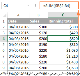
Excel Cumulative Sum formula

In a similar manner, you can use the Excel SUM function to find the cumulative sum for your bank balance. For this, enter deposits as positive numbers, and withdrawals as negative numbers in some column (column C in this example). And then, to show the running total, enter the following formula in column D:

=SUM($C$2:C2)
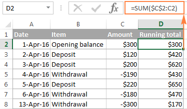
Calculating running total for the bank balance

Strictly speaking, the above screenshot shows not exactly a cumulative sum, which implies summation, but some sort of "running total and running difference"  Anyway, who cares about the right word if you've got the desired result, right? :)

At first sight, our Excel Cumulative Sum formula looks perfect, but it does have one significant drawback. When you copy the formula down a column, you will notice that the cumulative totals in the rows below the last cell with a value in column C all show the same number:
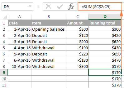
The cumulative totals in the rows below the last cell with a value in the dependent column all show the same number.

To fix this, we can improve our running total formula a bit further by embedding it in the IF function:

=IF(C2="","",SUM($C$2:C2))

The formula instructs Excel to do the following: if cell C2 is blank, then return an empty string (blank cell), otherwise apply the cumulative total formula.

Now, you can copy the formula to as many cells as you want, and the formula cells will look empty until you enter a number in the corresponding row in column C. As soon as you do this, the calculated cumulative sum will appear next to each amount:
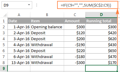
An improved Excel cumulative sum formula

How to make a cumulative graph in Excel

As soon as you've calculated the running total using the Sum formula, making a cumulative chart in Excel is a matter of minutes.

  1. Select your data, including the Cumulative Sum column, and create a 2-D clustered column chart by clicking the corresponding button on the Insert tab, in the Charts group:
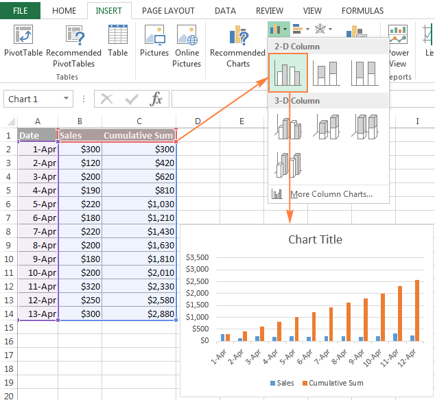
    Create a 2-D clustered column chart.
  2. In the newly created chart, click the Cumulative Sum data series (orange bars in this example), and right click to select Change Series Chart Type... from the context menu.
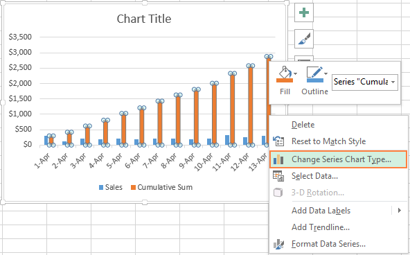
    Select Change Series Chart Type... from the context menu.
  3. If you are using a recent version of Excel 2013 or Excel 2016, select the Combo chart type, and click on the first icon (Clustered Column - Line) at the top of Change Chart Type dialog:
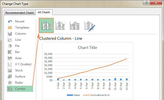
    In Excel 2013 or Excel 2016, select the Combo chart type.

    Or, you can highlight the Custom Combination icon, and choose the line type you want for the Cumulative Sum data series (Line with Markers in this example):

    Choose the line type you want for the Cumulative Sum data series.

    In Excel 2010 and earlier, simply select the desired line type for the Cumulative Sum series, which you've selected on the previous step:

    In Excel 2010 and earlier, select the desired line type for the Cumulative Sum series.

  4. Click OK, and evaluate your Excel cumulative chart:
    Excel cumulative chart
  5. Optionally, you can right-click the Cumulative Sum line in the chart, and select Add Data Labels from the context menu:
    Add data labels to the Cumulative Sum line.

As the result, your Excel cumulative graph will look similar to this:
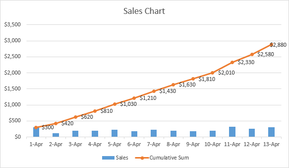
Excel cumulative graph with data labels

To embellish your Excel cumulative chart further, you can customize the chart and axes titles, modify the chart legend, choose other chart style and colors, etc. For the detailed instructions, please see our Excel charts tutorial.

This is how you do a running total in Excel. If you are curious to learn a few more useful formulas, check out the below examples. I thank you for reading and hope to see you again soon!

96 comments

  1. Hi
    ColumnA has for the date value and column B has cumulative value, if we enter the for the date value in column A, automatically the cumulative value will reflect in column B.

    Is there any formula for this kindly guide me

    • Hi,
      I’m sorry but your task is not entirely clear to me. For me to be able to help you better, please describe your task in more detail. Please specify what you were trying to find, what formula you used and what problem or error occurred.
      It’ll help me understand it better and find a solution for you.
      But you can automatically insert a value into a blank cell only with a VBA macro

  2. Is there a way to pull a specific date based on the cumulative total. As in, when did the total pass $1700? Is there a function to return that date?

    I am working on a data set where I am projecting X number of real estate developments per year. Lets say at 6 per year. I want to show in what year that the total passes development 14 is built? (This would be year 3). I cannot figure out the function.

    Thanks!

    • Hello!
      Column A contains dates, column B - amounts, column C - cumulative total. The date when the cumulative total exceeded a certain amount can be determined by the formula

      =INDEX(A1:A100,MATCH(1700,C1:C100,1)+1)

      Hope this is what you need.

  3. .Range("L8").Formula = "=IF(AND(F5="",G5="",H5=""),"",I4+F5-G5-H5)" ehy its not work can anyone help

    • Hello!
      Without seeing your data it is difficult to give you any advice. Please describe in more detail what problem you are having with this formula. What does not work?

  4. Thank you for this info - got me going quickly with a spreadsheet I needed in a hurry!
    -- Steve

  5. i am looking to complete the following task.
    row of cells that have a pass or fail drop down option. i have a running total of each but need to work out a way for an aditional cell to feep a running total even when the original cells in the row are cleared and a new option selected. So trac the overall passes and fails as the cells are used multiple times. Is this possible?

  6. Hi Everyone,

    I am looking to calculate a maximum cumulative average of at least 60 cells in length from within a larger range of cells. So, if in a range of data (A1:A101), with the cumulative average running from cell A1 to cell A101, how would I find out the section within this range that has the highest cumulative average? To qualify, it has to be at least 60 cells long.

    Thank you

    • Based on 100 rows of data -
      In column B, work out the average for your range,
      so
      B1 = =Average(B1:B60)
      B2 - =Average(B2:B61)

      Continue this down for 41 rows so all accumulations are covered.

      In column C, use the Rank option to see which set is the highest/lowest group of values.
      = B1 =RANK(B1,$B$1:$B$41,0) all the way down to C40
      This will give you the highest ranked, =RANK(B13,$B$1:$B$41,1) Changing the 0 to a 1 will give you the lowest ranked.

  7. I'm creating a spread sheet to track provisional credit issued and then funds recouped. What I want to be able to do is enter a total into column A say 200.00 then in column B enter the return credit of 50.00 and have that amount auto subtract so that column A now reads 150.00.

    To further complicate it in rare situations I have a third column C where I will on occassion need to subtract from column B without impacting the total in column A. So if I put 25.00 in column C. Column B becomes 25.00 but column A stays 150.00.

    • Hello Kristin!
      If a value is written in cell A1, then the formula can no longer be written to it. This has already been discussed on the blog many times. So your question about the formula in cell A1 does not make sense. Only VBA Macro Can Solve the Problem

  8. Hi,
    I have 2 columns.
    First column is text of various items , with varying amounts of the same items (1-100).
    Second column is just numbers relating to data in first column.
    I am trying to get a running total in the second column for each item in the first column.
    Any help appreciated.

    • Hello Alan!
      If I understand your task correctly, if the name of the item is recorded in column A, the quantity is recorded in column B, then running total can be calculated by the formula

      =SUMIF($A$3:A30,A3,$B$3:B30)

      I hope my advice will help you solve your task.

  9. ABoslutely saved me! Very much useful. Thanks a lot

  10. Hello,

    Can you explain how to run totals in different years? When I do it, it simply starts over for each year. Example;
    Quarters Data per quarter Increasing and Expected Result Actual result
    Q1 2019 10 10 10
    Q2 2019 5 15 15
    Q1 2020 6 21 21
    Q2 2020 3 24 24
    Q1 2021 1 25 1
    Q2 2021 2 27 3

    How can I achieve the increasing and expected result values?

  11. thank you so much! this helped a ton!

  12. thank's for your help but there is another issue when I tried to select the cell and didn't go well, but it worked eventually

  13. Hi,
    Simple solution for everything. please swtichoff your system and sleep.

  14. I have my weekly expenses totalled and each week has different items listed with a final total for the week. what I want to do is over the year I want a total of each weeks totals to give me a total for the year. e.g. I want a total for say P15+P30+P45 etc. I have a basic knowledge of excel but this has beaten me. Please Help.

  15. Thanks very much for tutorials, I like to know if there is a way to make just a cell behave as a normal calculator.
    i.e this cell should be capable of summing figures that appears in another cell, while keeping last cumulative figure visible.
    This other cell will be the key-in cell or active cell.
    Example:
    Cell 1: =2*5, Answer appears in Cell 2,
    Cell 1: =3*6.8, Answer is added to the previous value resulting from (2*5) and still appears in cell 2.
    Kindly share a video if this is possible.
    Thank you.

  16. Veryful, thank you

  17. Thanks you saved me a ton of time with the cumulative sum formula :)

  18. Let's say I want cell B2 to be a cummulative total of minutes that only accumulates if cell A2 matches with the same name I select from a dropdown list in cell D2. Can this be done? Example: Cell A2(A constant) contains T Young, then Cell D2 from a drop down list has T Young selected. Then Cell E2 has a number entered that I want added only to the running total of minutes in Cell B2, only if cells A2 and D2(Dropdown List) match.

  19. Wonderful, I'm grateful

  20. Hi
    I am trying to do a running total of collum M in Collum P. I have managed to do this using you help. Now i need to take away collum O and keep the running total going in Collum P

    PLEASE HELP its doing my head in.

  21. What about a formula where a number is entered in a cell and other cells subtract the new increment from their previous total? Not the total in the 1st cell, but the new number added to it. I'm trying to keep it from becoming a list, as with expenses.

  22. I am trying to set up a running total of total hours worked and total dollars in labor. So that each week I will change the weekly numbers but need it to be added as I go from week to week in another column. What formula will work for this? I am not having any luck. All the formulas I am finding want the week to week numbers to be kept and then added as a running total. I need the running number to keep adding as the weekly numbers change.

  23. if $ sign is used, what happens if a new column is inserted to the left.

    • Absolute cell references (with the $ sign) do change when you add or remove rows and/or columns to reflect a new position of the referenced cell, so your reference will change accordingly.

  24. Hi There,
    I am doing a rota at work for around 50 staff. I want to know how do I set up a total figure for individuals holidays as they are booked so a running total of what they have left for the year is displayed.
    I insert the letter H on the rota if a holiday is booked.
    Hope you can help

    Thank you

    Jethro

  25. I am a person looking for a probability function in a distribution where one has to make Cumulative functions as well as probability ranges!

  26. Hi there,

    My request is complex (well, I think so). I am looking to do a running total of the number of equipment used in a period of dates.

    If I have in total: 100 bikes
    Shop A with 50 bikes
    Shop B with 30 bikes
    Shop C with 20 bikes

    In the week of March 1-6, Shop A will use 30 bikes, B will use 10 bikes and C will use 5 bikes, is there a way of determining how many bikes are being used in March 1-6 across all three sites?
    This will also be able to produce an error/warning if I may be using more than 100 bikes.

    I would imagine that I have start and end dates in a particular format so that I can use an sumif() function to calculate the sum of bikes in a particular week. Does that sound right?

    Happy to discuss through private email.
    Thanks

  27. I have columns with different items and then prices and then a total what I want is for it to automatically sum up the total of the previous square with the new amount put in. For example
    B C D E
    ITEM, DESCRIPTION, AMOUNT, TOTAL
    Food, Bagel , $3.00, =$3.00
    Drink, Tea ,$ 2.00, =$5.00 etc...

    But I want it to sum it up automatically, right now I am having to do it individually =SUM(E1,D2) can anyone help?

    • Hello,

      If I understand your task correctly, please try to do the following:

      1. Enter the following formula in cell E2;

      =SUM($D$2:D2)

      2. Just select the cell where you've entered the formula and drag the fill handle (a small square at the lower right-hand corner of the selected cell) down.

      Hope this will help.

  28. how to sum multiple cell in sum if formula

  29. I have been adding expenses in a column in Excel using the Summation function showing at the BOTTOM of a column of data.
    Whenever I have to add a new expense, I simply add a row and then enter the datum.
    However, upon returning to the expensive file/column recently, I noticed that somewhere during the middle of the year the column started adding a cumulative data amount, over-writing the entry I added for the individual expense.
    I tried clearing "format" to see if it would return the original data entry. I can see that the cell below (e.g. C24 was originally C24-C23. Yikes! How can I go back to original summary cell at the bottom of my column, and undo the cumulative summation/overwrite that somehow is at play? Thank you.

    • Hello,
      For me to understand the problem better, please send me a small sample workbook with your source data and the result you expect to get to support@ablebits.com. Please don't worry if you have confidential information there, we never disclose the data we get from our customers and delete it as soon as the problem is resolved.
      Please also don't forget to include the link to this comment into your email.
      I'll look into your task and try to help.

  30. my sheet column head is description (A:A), debit(B:B), credit(C:C), Balance (D:D). In description if i write "Deposit" then the value will put on debit column, and if write "Credited", the value will put on credit column. But how to ensure if i write "credit" in A3, THE VALUE 500 will only can be post in Credit column C3, B3 should not accept any input if the description is 'CREDITED'. OR if the description is "deposit" the value cannot be post in Credit clumn C3. How to apply, pls.

    • Hello,

      If I understand your task correctly, please create a custom Data Validation rule for columns B and C using these formulas:

      column B
      =A1="Deposit"

      column C
      =A1="Credited"

      We have an article on our blog that describes how to use Data Validation in Excel. Please have a look at it.

      Hope you’ll find it helpful.

  31. This was an elegant and efficient solution, thanks

  32. i need a formula to get ending balance of today then that ending balance will be the beginning balance the next day. thank you.

    • I’ve been trying to figure out how to do this as well. Have you got your answer?

  33. Hi,
    I need to calculate the rate of an electricity bill but the tariff is accumulative so if I have 5,000 unit the first 1,000 is at certain price the the second 1,000 at a different price and so on. can I make a formula in Excel to segregate the total units number and calculate each part at a different rate.

  34. I need a formula that sums a column up to $250 then stops the sum and starts listing the amount in the cell.

    This formula got me started =IF(SUM($E$4:E11)>$F$1, ,SUM($E$4:E11)-250)

    • Hello, Charles,

      I'm sorry, I'm afraid your task is not entirely clear.
      If you still need assistance with it, please email us your Excel table with the data and the result you expect to get to support@ablebits.com. Don't forget to link this comment.

  35. How do we handle when instead of sales in units ? for example the weekly budget is 130 and weekly sales for week 1 -133 week 2- 133, week 3-133 week 4- 134 week 5 -135 so whats happening here is in week 1 it will be +4 and should be +4 for week 2 and 3 because in actuality we are not selling more units. Further when we come to week 4 the increase is just 1 unit in sales so do we add 4 from prior week and 1 from current week to show 5 units or will it be 4+5 units in cummulative ? This is a case of addition but when there is a deficit vs the budget we have to add the negative units from prior period to current period so either it can net off against the surplus or add to more deficit.

    • Weekly budget is 129 not 130.

  36. How to check particular row cumulative result in a column using cumulative addition

  37. How to display running total in a cell. For example: you want cell E1 to display the newest ever chaning running total in above diagram $170 from column D.

  38. hi guys! how do I run a cumulative sum of a previous cell value with the current cell value is a different cell? I.e previous value of A1 current value of A1 in B1

  39. Thank you so much for this information. I have been wanting to learn how to create a cumulative graph for quite some time now, and these instructions are wonderful. I do, however, have a question:

    I successfully created a cumulative graph based on hours entered in time sheets by a particular role of employee. My problem is that the dates for time entry are daily, and the project has been running for a long time. This makes the graph impossible to read. Is there a way to change the time increment to monthly instead of daily? This would help tremendously!

  40. Thank you so much for the explanation. That was very clear and helpful.

    Regards
    Rajen Appadoo

  41. Hi,

    I have 5 worksheets, 2 with weekly wages for 2016 & 2017 and two with weekly revenue for 2016 & 2017 and I have setup another worksheet which gives me what revenue/wages was for both years by putting in a week number in a cell (done by hlookup )
    What I need is a cumulative figure for the year depending on what week we are in. ie if I put in wk 9 in my cell, that It will cumulative the first 9 weeks of the year for the wages/revenue for 2016/2017 and not the total for all the weeks are have been entered.

    Kind regards,

    Padraig

  42. I have 3 coloumn , abc,a coumn heading date,b col party name,c column amt,d columns balance d1 only want to see i i entetd anydate in a columns,add amt im d1 cell automatically how can i do this,=if(blank(),sum(c comumn row 1,2,3,4,..... in only d 1 cell only when we enterd date in columns a1 to a12 for exanple.we guide me

  43. Good tips. I love it.

  44. Hi!

    Im having hard time formulating the beginning balance on a selected period of a cash flow. For example, i would like to filter only the transaction of yesterday or the other day, but i dont know how to formula the beginning balance of that period.

    Do you have a preferred excel formula to be used on this problem?

    Thank you.

  45. I have an spread sheet in excel 10 with 23 sheets and a summary sheet.

    I have a running balance set up on the 23 sheets using tables referencing system called structured references. The formula in the balance column is =SUM(INDEX([Debit],1):[(@Debit])-SUM(INDEX([Credit],1):[2Credit]).
    This produces a running balance for each sheet.

    I can get data into the summary sheet by using =[Sheet Name]![Cell]but that only references the first cell.

    What I need to know is how to get the relevant cell in the summary sheet to update as the data in the corresponding cell is changed with each input entry.

    The idea is, I start with an opening balance, enter debits or credits, a new balance is created and updated in the summary sheet. Next time I open the spread sheet I simply enter new data and the new balance is updated in the summary sheet each time I make changes.

    I trust you are able to help and I await you advice in due course.
    Peter.

    • Hi Peter,
      I am trying to do a similar thing. Did you get an answer to your question?
      Thank you,
      Janet

  46. Is there a way to run the IF formula on multiple cells? Example you have =IF(C2="","",SUM($C$2:C2)) to return a blank cell unless something is in C2. What if I have a column c2, d2 and e2, and want it to return a value if only 1 of those columns is filled it?

  47. How do I calculate sales for many different products and total per state- soo all sales for each state not broken out by product

  48. I have been having trouble understanding exactly how to work out this cumulative sum until I met it in your web. Its all clear to me now. Thanks.

  49. I am not skilled in excel whatsoever. Sorry. What I'm needing is to make Column A + Column B + Column C = Column D, and make it average out the sums from Column D in Column E

    • For example
      In Cell D3 write:

      =SUM(A3:C3)

      fill down. Then in Cell E3 write:

      =AVERAGE(A3:C3)

      also fill down.

  50. Thank u so much for great information
    Keep it up

    Regards
    Saurabh

Post a comment


Thank you for your comment!
When posting a question, please be very clear and concise. This will help us provide a quick and relevant solution to
your query. We cannot guarantee that we will answer every question, but we'll do our best :)