Want to know how many characters there are in a certain cell? This tutorial will help you choose an Excel formula for character count best suited for your particular case.
Initially, Excel was designed to work with numbers. Fortunately, the developers of this helpful application didn't forget about text. Below, you'll find a number of formulas for counting characters in Excel. Just look through the examples and see which one best suits your needs.
Here are the cases we are going to cover:
Excel formula to count the number of characters in a cell
First things first, let's solve the most common case. To find how many characters there are in an Excel cell, the formula is as simple as:
For example, to count characters in each cell of column A beginning in A3, this is what you need to do:
- Enter the below formula in any empty cell in row 3:
=LEN(A3) - Double-click the fill handle to get the formula copied across the whole column.
Done!
Feel free to use this formula each time you need to count the number of characters in a string.
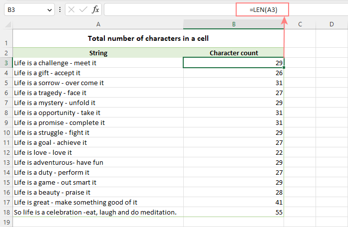
Note. Please pay attention that the Excel LEN function counts absolutely all characters in a cell, including letters, numbers, punctuation marks, special symbols, and all spaces (leading, trailing and spaces between words).
Count characters in a range of cells
To get the total of characters in an Excel range, you can use the LEN function together with SUMPRODUCT:
And your real-life formula may look similar to this:
=SUMPRODUCT(LEN(A3:A18))
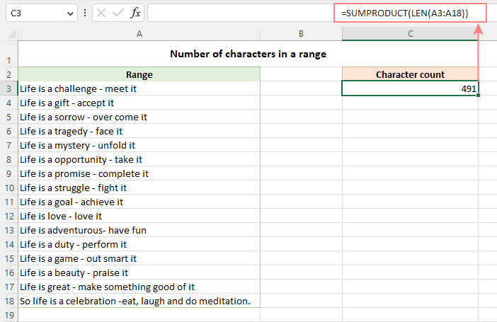
Another way to count all characters in a range is using LEN in combination with the SUM function:
=SUM(LEN(A3:A18))
Unlike SUMPRODUCT, the SUM function does not process arrays by default, so you need to press Ctrl + Shift + Enter to turn it into an array formula in Excel 2019 and earlier. In Excel 365 and 2021, it works as a regular formula due to inbuilt support for dynamic arrays.
How this formula works:
The logic is very simple. The LEN function calculates the string length for each individual cell in the specified range and returns an array of numbers. And then, SUMPRODUCT or SUM adds up those numbers and returns the total character count.
How to count specific characters in a cell
To find out how many times a given character appears in a cell, the generic formula is:
Suppose you maintain a database of items where each item type has its own unique identifier. And each cell contains several items separated by comma, space, or any other delimiter. The task is to get the number of occurrences of a certain unique identifier in each cell.
Assuming the list of items is in column A beginning in A3, and the target character is in column B in the same row, the formula is as follows:
=LEN(A3) - LEN(SUBSTITUTE(A3, B3, ""))
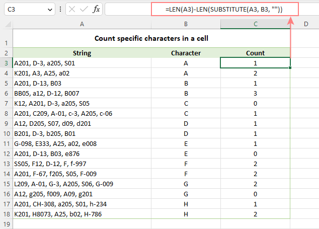
Note. Excel's SUBSTITUTE is a case-sensitive function, and therefore the above formula treats uppercase and lowercase letters as different characters. For example, cell A4 in the screenshot above contains one occurrence of "a" and two occurrences of "A". The formula counted only the uppercase "A" and returned 2 as the result.
How this formula works:
To understand the formula's logic, let's break it down into smaller parts:
- First, you find the total string length in cell A3 with:
LEN(A3) - Then, you remove all occurrences of the letter "A" in A3 by replacing it with an empty string:
SUBSTITUTE(A3, "A", "") - The next step is to find the string length without the letter "A":
LEN(SUBSTITUTE(A3, "A", "")) - Finally, you subtract the length of the string without "A" from the total length string:
LEN(A3) - LEN(SUBSTITUTE(A3, B3, ""))
As the result, you get the count of "removed" characters, which is the number of occurrences of that particular character in the cell.
Case-insensitive formula to count letters in Excel cell
When counting letters in Excel cells, you may sometimes need a formula that ignores the letter case. To make such a formula, use the UPPER function inside SUBSTITUTE to convert a given letter to uppercase before running the substitution.
For example, to count both "A" and "a" in cell A3, use this formula:
=LEN(A3) - LEN(SUBSTITUTE(UPPER(A3), "A", ""))
The LOWER function will also do:
=LEN(A3) - LEN(SUBSTITUTE(LOWER(A3), "a", ""))
A slightly more complex way is using nested SUBSTITUTE functions:
=LEN(A3) - LEN(SUBSTITUTE(SUBSTITUTE (A3, "A", ""), "a", "")
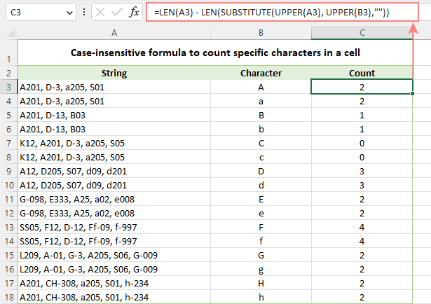
In our data set, the letters to be counted are input in column B, so we convert both the source cell and the cell containing the character to uppercase:
=LEN(A3) - LEN(SUBSTITUTE(UPPER(A3), UPPER(B3),""))
And this works beautifully irrespective of the target letter's case:
How to count certain text/substring in a cell
If you want to know how many times a certain combination of characters appears in a given cell (e.g. "C2" or "C-2" or "cat"), then divide the characters count by the length of the substring.
Case-sensitive formula:
=(LEN(A3) - LEN(SUBSTITUTE(A3, B3, ""))) / LEN(B3)
Case-insensitive formula:
=(LEN(A3)-LEN(SUBSTITUTE(UPPER(A3), UPPER(B3),""))) / LEN(B3)
Where A3 is the original text string and B3 is the substring to count.
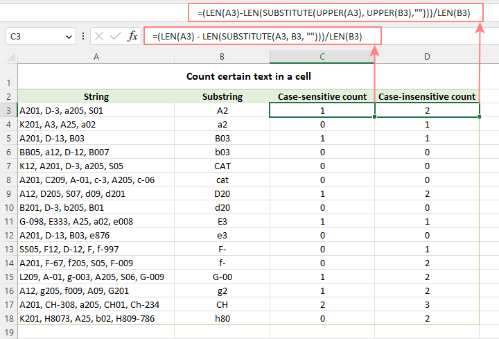
For the detailed explanation of the formula, please see How to count specific text / words in a cell.
How to count specific characters in a range
Knowing a formula for counting certain characters in a single cell, it's quite easy to modify it a little further to count the number of occurrences of a given character in several cells. For this, just place the LEN formula inside the SUMPRODUCT function that can handle arrays:
For example, to get to know how many times the character in D2 occurs in the range A3:A18, the formula is:
=SUMPRODUCT(LEN(A3:A18) - LEN(SUBSTITUTE(A3:A18, D2, "")))
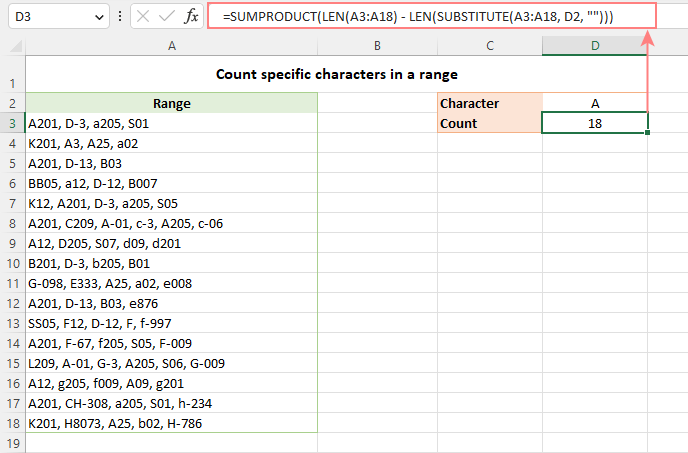
Instead of SUMPRODUCT, you can also use SUM:
=SUM(LEN(A3:A18) - LEN(SUBSTITUTE(A3:A18, D2, "")))
But this formula requires pressing Ctrl + Shift + Enter because, in all versions other than Excel 365 and 2021, SUM can handle arrays only in an array formula.
How this formula works:
The SUBSTITUTE function replaces all occurrences of a given character ("A" in this example) with an empty string ("").
The text string returned by SUBSTITUTE is served to the LEN function so it calculates the string length without A's.
The string length without A's is subtracted from the total length of the original string. The result is an array of character counts per cell.
Finally, SUMPRODUCT sums the numbers in the array and returns the total character count in the range.
Case-insensitive formula to count letters in a range
To create a case-insensitive formula for counting specific characters in a range, follow the same approaches that we used for counting certain letters in a cell regardless of the text case.
Use the UPPER function and supply an uppercase letter:
=SUMPRODUCT(LEN(A3:A18) - LEN(SUBSTITUTE(UPPER(A3:A18), "A", "")))
Use the LOWER function and supply a lowercase letter:
=SUMPRODUCT(LEN(A3:A18) - LEN(SUBSTITUTE(LOWER(A3:A18), "a", "")))
Nest a couple of SUBSTITUTE functions one into another:
=SUMPRODUCT(LEN(A3:A18) - LEN(SUBSTITUTE(SUBSTITUTE((A3:A18), "A", ""), "a", "")))
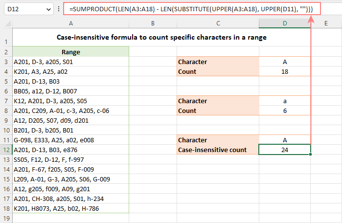
In the character of interest is input in a predefined cell, UPPER or LOWER will work equally well:
=SUMPRODUCT(LEN(A3:A18) - LEN(SUBSTITUTE(UPPER(A3:A18), UPPER(D2), "")))
Or
=SUMPRODUCT(LEN(A3:A18) - LEN(SUBSTITUTE(LOWER(A3:A18), LOWER(D2), "")))
The below screenshot shows it in action:
How to count certain text / substring in a range
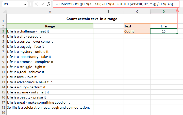
To count the number of occurrences of certain text in a range, use this generic formula:
For example, to count the number of times the word "Life" appears in the range A3:A18, the formula is:
=SUMPRODUCT((LEN(A3:A18) - LEN(SUBSTITUTE(A3:A18, D2, ""))) / LEN(D2))
Excel character limits for cells
Microsoft Excel has a limitation on the number of characters that can be entered in a cell. If you have worksheets with large amount of text data, you may find the following information helpful.
- The total number of characters that a cell can contain is 32,767.
- A cell can only display 1,024 characters. At the same time, the Formula bar can show all 32,767 symbols.
- The maximum length of a formula is 8,192 characters in Excel 2007 and higher (1,014 in Excel 2003).
Please consider the facts when you are going to merge or import data from an external source.
These are the best practices for counting characters in Excel. For first-hand experience, you can download a sample workbook and check out a list of related resources at the end of the page. Thank you for reading and hope to see you soon!
Practice workbook for download
Count characters in Excel - formula examples (.xlsx file)
 by
by
147 comments
I Wish to get number value (example 5) in B1 cell from √ symbol in A1 cell
formula worked fine but is not constant in the next cell below..... why is that. may I know how to let all the cells below function the same way I commanded the first cell above.
if my cell is like below
1,AF
and I need to count " AF " is that possible to do? how? what formula will I have to use?
Thank you.
Hi guys,
I have two columns in my spreadsheet - code(1-18) and duration in minutes (1-300)
I need to get the sum of values(values in minutes) of the same code of cells. The code still in numbers (eg 1-18)
Kindly someone help.
I'm creating a spreadsheet (Excel 2003) in which a user enters data in several cells, each of which will permit only 50 numbers of characters (to include spaces). i have used data validation to limit cahracters to 50, but i want to show number of characters typed simultaneously. anyone please help me out. thanks in advance.
12251197-ltc-mun-transporte-ejecutivos-oriente-anibal-golindano-1900006354-m-i-swaco.xls
12238385-ben-chalbi-faical-3028438-wireline.xls
i want to find employee no which is stat with 1900 and does not start with 1900.
how can i want find both in one formula.
I have cells with part numbers, I.E.
123456-1
123456-2
24W652-1
24W652-2
etc.
I need formulas to find out how many odd numbers and even numbers I have total as they equate to left and right sides of an aircraft?
Hello, Gary,
Please use the following formula for the odd numbers:
=SUM(--(MOD(1*RIGHT(A1:A7,1),2)=1))
The one for the even numbers:
=SUM(--(MOD(1*RIGHT(A1:A7,1),2)=0))
Here A1:A7 is your list address. Please note that these formulas are array formulas. Use Ctrl + Shift + Enter to enter them.
Hi guys,
I am using Excel 2010.
I'd like to ask you for your kind support. I am looking for formula which calculate with text & no. (where no. is changing).
Example:
A1=R00000
I need to get in A2=A1+1 --> R00001
Thank you in advance.
Milan
I'm struggling to count a specific alphabet like "P" in a cell range of a few words.
Hi Thibolover,
Check out the following example:
Array formula to count any given character(s) in a range
I know how to count a "V" in a cell for one, but I was wondering if there is anyway I can count it as .5 and as 1 too. What can I put to make it count as .5?
843,138FS+5d,411,416,766,132
41
42
43
44
83,81,45
46
70
90SS
399
97
98SS
99SS
100SS
101SS
130
131
834,134
141
544FF,531FF,558FF,761FF,560FF,570FF,555FF,551FF
Each of these is in a separate cell, I'm trying to count those without SS or FF on the end. This is to count the number of FS relationships in an export from MS Project. I have been able to do the count of SS and FF.
Hello, Carla,
To help you better, we need a sample table with your data in Excel. You can email it to support@ablebits.com. Please add the link to this article and your comment number.
hi,
i want to enter a number and after that some information appear.for example when i enter 570, after that some information in a row about weight,quality,tonnage or other things should provide. i use the custom list in excel option but the error (cells without simple text were ignored) appear. what should i do???
please help me
thank you
Where I work we have to maintain a daily census that lets us know how many people are in the building, including residents and guests.
I want to know if I when a name is added or removed how can I keep a running total.
So in other words to make sure I am explaining myself, if a resident moves in, or passes away, or is in the hospital or a family member stays with us we have to know how many people (not staff) or in the building. So if right now I have 70 residents and tomorrow one goes to the hospital and one moves out my total should say 68. So how to I get the 70 to change from 68 using names of people not numbers. Right now if someone forgets to change the total manually then we could have problems. But if the number changes with a name added or removed it would help a lot. Thank you.
How do I separate the text for the following
hienze/adsfdsaf kt/feD.xl - "i need "feD.xl" in this
asda/sfer/aedfew/rwtw/sdfjhk.cl - "i need "sdfjhk.cl" in this"
ewr/tye.tre - "i need "tye.tre" in this"
Basically i need to get the text after the last "/" in every cell.
Appreciate your help
Thanks
how to count only text.
question
1
2
d
d
e
3
2
2
d
Now please count only text value. I tried but it counts space also.
In an excel spreadsheet, if I have 5 cells in a row or column, 4 cells which have a number value and only one cell that has a text format, such as a name, how do I create a formula that will ignore cells with numbers and input the only text value as my answer?
For instance,
If C1 = 4, C2 = 6, C3 = 9, C4 = Quality Paving, C5 =2
And I created a formula in another cell, such as Cell D14, with formula, =Sum(C1:C5), my value would be the sum of all the numbers. But I want my value in a certain cell to equal Quality Paving. What formula can you create that will ignore the number cells and give you the text value only as it is in another cell?
Hi,
Good information but i need additional help for filtered columns...
I am trying to count the number of cells that have "X" (the X comes from a formula where the cell has this then an X goes into this cell (=IF(X1="LTI","X","")) in them but the column is filtered by year or month. So i only want to count the cells containing an X if they are displayed when filtered.
really struggling with this.
thanks
Hello, Brad,
Here's the fomula:
=SUMPRODUCT(SUBTOTAL(3,OFFSET(A1:A10,ROW(A1:A10)-MIN(ROW(A1:A10)),,1)),ISNUMBER(SEARCH("X",A1:A10)) + 0)
hi,
I have a one problem which I can't solve. I have about 10 sheets in one excel and in every sheet is an table which contain a rows with text. In the laste sheet I would like to summarize the whole from sheets but I don't know which formula I can use for do this. I want to count or sum the text accross the multiple sheets but I don't know how. Thanks for response!
Hello, Valentina,
You need to add the references to other sheets. For example, here the formula for the number of text cells from 3 sheets (Sheet1, Sheet2, Sheet3) with data in A1:A10:
=COUNTIF(Sheet1!A1:A10, "*") + COUNTIF(Sheet2!A1:A10, "*") + COUNTIF(Sheet3!A1:A10, "*")
Ms. Maria Azbel:
What if you have a variety of names (instead of sheet 1, Sheet2)on your multiple sheets and you want to count or sum the text across those multiple sheets from one column; could you not use a formula that is like the First Last formula? =SUM(First:Last!D28)
Would I do: =COUNTIF(First:Last!D28) ?
hi
would you please help me to find a equation in excel i have tried many times to find it i could not find. in a column there are different texts there are "/" in middle of some texts i want to avoid some letters from that texts that letters beyond the "/" and include "/" .i want to change below texts like
eg: han/han han
pan/san pan
ran/man ran
Use this formula considering the values start from cell A1, B1 and so on:
=LEFT(A1,FIND("/",A1)-1)
This formula finds the "/" character and displays all the text till that character and the "-1" removes the "/" character
How do I separate the text for the following
hienze/adsfdsaf kt/feD.xl - "i need "feD.xl" in this
asda/sfer/aedfew/rwtw/sdfjhk.cl - "i need "sdfjhk.cl" in this"
ewr/tye.tre - "i need "tye.tre" in this"
Basically i need to get the text after the last "/" in every cell.
Any help will be highly appreciated
This should work. I've written it as though your data begins in cell A1. Copy this formula down.
=SEARCH("^",SUBSTITUTE(A1,"/","^",LEN(A1)-LEN(SUBSTITUTE(A1,"/",""))))
Whoops, I left out the piece before "SEARCH"...
=RIGHT(A1,LEN(A1)-SEARCH("^",SUBSTITUTE(A1,"/","^",LEN(A1)-LEN(SUBSTITUTE(A1,"/","")))))
Hi Maria I have tried your solutions but in all cases where im trying to count cells with text in the formulas seems to include cells with formulas in, I have 1400 rows and I want to count the number of cells that match my formula IF(ISERROR(MATCH *** . the formula im using works as it compares names in two columns but now I want to total it up and all i get using your ideas it is the full row total. Is there a way of doing this and ignoring cells with formula ?
simple =len(text)