In this article, you will learn new effective approaches to summing and counting cells in Excel by color. These solutions work for cells colored manually and with conditional formatting in all versions of Excel 2010 through Excel 365.
Even though Microsoft Excel has a variety of functions for different purposes, none can calculate cells based on their color. Aside from third-party tools, there is only one efficient solution - create your own functions. If you know very little about user-defined functions or have never heard of this term before, don't panic. The functions are already written and tested by us. All you need to do is to insert them in your workbook :)
How to count cells by color in Excel
Below, you can see the codes of two custom functions (technically, these are called user-defined functions or UDF). The first one is purposed for counting cells with a specific fill color and the other - font color. Both are written by Alex, one of our best Excel gurus.
Once the functions are added to your workbook, they will do all work behind the scenes, and you can use them in the usual way, just like any other native Excel function. From the end-user perspective, the functions have the following look.
Count cells by fill color
To count cells with a particular background color, this is the function to use:
Where:
- Data_range is a range in which to count cells.
- Cell_color is a reference to the cell with the target fill color.
To count cells of a specific color in a given range, carry out these steps:
- Insert the code of the CountCellsByColor function in your workbook.
- In a cell where you want the result to appear, start typing the formula: =CountCellsByColor(
- For the first argument, enter the range in which you want to count colored cells.
- For the second argument, supply the cell with the target color.
- Press the Enterkey. Done!
For example, to find out how many cells in range B3:F24 have the same color as H3, the formula is:
=CountCellsByColor(B3:F24, H3)
In our sample dataset, the cells with values less than 150 are colored in yellow, and the cells with values higher than 350 in green. The function gets both counts with ease:

Count cells by font color
In case your cell values have different font colors, you can count them using this function:
Where:
- Data_range is a range in which to count cells.
- Font_color is a reference to the cell with the sample font color.
For example, to get the number of cells in B3:F24 whose values have the same font color as H3, the formula is:
=CountCellsByFontColor(B3:F24, H3)
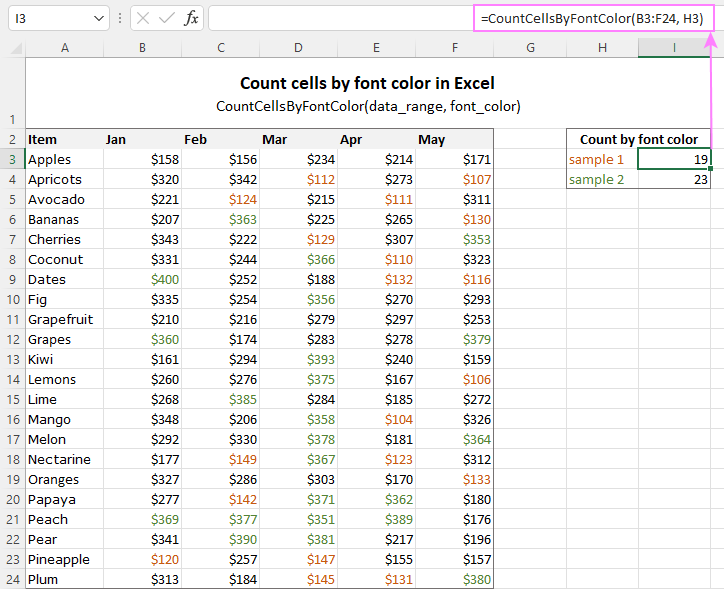
Tip. If you'd like to name the functions differently, feel free to change the names directly in the code.
How to sum by color in Excel
To sum colored values, add the following two functions to your workbook. As with the previous example, the first one handles fill color and the other - font color.
Sum values by cell color
To sum by fill color in Excel, this is function to use:
Where:
- Data_range is a range in which to sum values.
- Cell_color is a reference to the cell with the fill color of interest.
For example, to add up the values of all cells in B3:F24 that are shaded with the same color as H3, the formula is:
=SumCellsByColor(B3:F24, H3)

Sum values by font color
To sum numeric values with a specific font color, use this function:
Where:
- Data_range is a range in which to sum cells.
- Font_color is a reference to the cell with the target font color.
For instance, to add up all the values in cells B3:F24 with the same font color as the value in H3, the formula is:
=SumCellsByFontColor(B3:F24, H3)
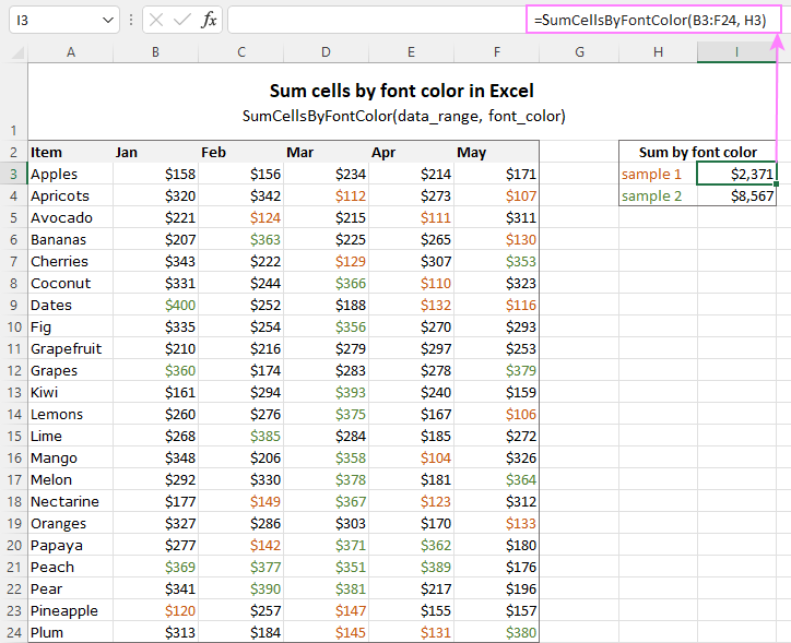
Count and sum by color across entire workbook
To count and sum cells of a certain color in all sheets of a given workbook, we created two separate functions, which are named WbkCountByColor and WbkSumByColor, respectively. Here comes the code:
Note. To make the functions' code more compact, we refer to the two previously discussed functions that count and sum within a specified range. So, for the "workbook functions" to work, be sure to add the code of the CountCellsByColor and SumCellsByColor functions to your Excel too.
How to count colored cells in entire workbook
To find out how many cells of a particular color there are in all sheets of a given workbook, use this function:
The function takes just one argument - a reference to any cell filled with the color of interest. So, a real-life formula may look something like this:
=WbkCountByColor(A1)
Where A1 is the cell with the sample fill color.
How to sum colored cells in whole workbook
To get a total of values in all cells of the current workbook highlighted with a particular color, use this function:
Assuming the target color is in cell B1, the formula takes this form:
=WbkSumByColor(B1)
Count and sum conditionally formatted cells
The custom functions for adding up and counting color-coded cells are really nice, aren't they? The problem is that they do not work for cells colored with conditional formatting, alas :(
To handle conditional formatting, we have written a different code (kudos to Alex again!). It works well with both preset formats and custom formula-based rules. Contrasting with the previous examples, this code is a macro, not a function. The macro counts and sums conditionally formatted cells by fill color. Please insert it in your VBA Editor, and then follow the below instructions.
How to count and sum conditionally formatted cells using VBA macro
With the macro's code inserted in your Excel, this is what you need to do:
- Select one or more ranges where you want to count and sum colored cells. Make sure the selected range(s) contains numerical data.
- Press Alt + F8, select the SumCountByConditionalFormat macro in the list, and click Run.
- A small dialog box will pop asking you to select a cell with the sample color. Do this and click OK.
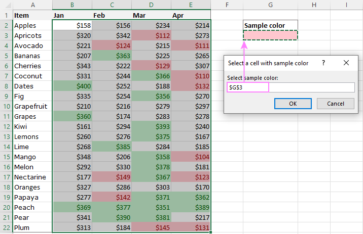
For this example, we used the inbuilt Highlight Cell Rules and got the following results:
- Count (12) the number of cells in range B2:E22 with the same color as G3.
- Sum (1512) is the sum of values in cells formatted with Light Red Fill.
- Color is a hexadecimal color code of the sample cell.
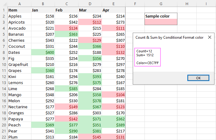
Tip. The sample workbook with the SumCountByConditionalFormat macro is available for download at the end of this post.
How to get cell color in Excel
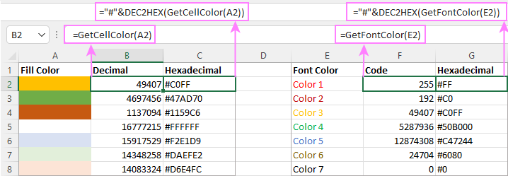
If you need (or are curious) to know the color of a specific cell (fill or font color), add the following user-defined functions to your Excel. It returns ColorIndex as a decimal number.
Note. The functions only work for colors applied manually, and not with conditional formatting.
Get fill color of a cell
To return a decimal code of the color a given cell is highlighted with, make use of this function:
For example, to get the color of cell A2, the formula is:
=GetCellColor(A2)
Get font color of a cell
To get a font color of a cell, use an analogous function:
For instance, to find the font color of cell E2, the formula is:
=GetFontColor(E2)
Get hexadecimal color code of a cell
To convert a decimal color index returned by our custom functions into a hexadecimal color code, make use of Excel's native DEC2HEX function.
For example:
="#"&DEC2HEX(GetCellColor(A2))
="#"&DEC2HEX(GetFontColor(E2))
How to insert VBA code in your workbook
To add the function's or macro's code to your Excel, move on with these 4 steps:
- In your workbook, press Alt + F11 to open Visual Basic Editor.
- In the left pane, right-click on the workbook name, and then choose Insert > Module from the context menu.
- In the Code window, insert the code of the desired function(s):
- Count by color: CountCellsByColor and CountCellsByFontColor functions
- Sum by color: SumCellsByColor and SumCellsByFontColor functions
- Count and sum colored cells in whole workbook: WbkCountByColor and WbkSumByColor functions
- Count and sum conditionally formatted cells: SumCountByConditionalFormat function
- Get color code: GetCellColor and GetFontColor functions
- Save your file as Macro-Enabled Workbook (.xlsm).
If you are not very comfortable with VBA, you can find the detailed step-by-step instructions and a handful of useful tips in this tutorial: How to insert and run VBA code in Excel.
How to get custom functions to update
When summing and counting color-coded cells in Excel, please keep in mind that your formulas won't recalculate automatically after coloring a few more cells or changing existing colors. Please don't be angry with us, this is not a bug in our code :)
The point is that changing cell color in Excel does not trigger worksheet recalculation. To get the formulas to update, press either F9 to recalculate all open workbooks or Shift + F9 to recalculate only the active sheet. Or just place the cursor into any cell and press F2, and then hit Enter. For more information, please see How to force recalculation in Excel.
Fastest way to calculate colored cells in Excel
If you do not want to waste time tinkering with VBA codes, I'm happy to introduce you to our very simple but powerful Count & Sum by Color tool. Together with 70+ other time-saving add-ins, it is included with Ultimate Suite for Excel.
Once installed, you will find it on the Ablebits Tools tab of your Excel ribbon:

And here is a short summary of what the Count & Sum by Color add-in can do:
- Count and sum cells by color in all versions of Excel 2016 - Excel 365.
- Find average, maximum and minimum values in the colored cells.
- Handle cells colored manually and with conditional formatting.
- Paste the results anywhere in a worksheet as values or formulas.
Sum and count cells by one color
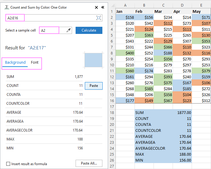
Selecting the Sum & Count by One Color option will open the following pane in the left part of your worksheet. You specify the source range and sample cell, then then click Calculate.
The result will appear on the pane straight away! No macros, no formulas, no pain :)
Apart from count and sum, the add-in also shows Average, Max and Min for colored numbers. To insert a particular value in the sheet, click the Paste button next to it. Or click Paste All to have all the results inserted at once:
Count and sum all colored cells at once
To handle all colored cells at a time, choose the Sum & Count by All Color option. Basically, it works in the same way, except that instead of color, you choose the function to calculate.
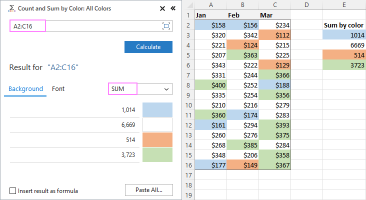
Tip. To have the results inserted in the worksheet as formulas (custom functions), check the corresponding box at the bottom of the pane.
Well, calculating colored cells in Excel is pretty easy, isn't it? Of course, if you have that little gem that makes the magic happen :) Curious to see how our add-in will cope with your colored cells? The download link is right below.
Available downloads
Sum and count by color in Excel - examples (.xlsm file)
Ultimate Suite 14-day fully-functional version (.exe file)
 by
by
791 comments
How to count by font colors, and within range, for example I only want to count, 12345, I only want to count 2 and 4, can I put ( "2")
I used this for a workbook with manually changed cell colours and everything is working but the numbers do not update when I change the cell colours. For example if I change one cell from green to blue, the count for each colour remains the same as it was before. Is there something I can do to fix this?
Code works flawless on how it's built. What I am trying add/change, is how can I "exclude" negative numbers?
Example code on one of my columns:
=SumCellsByColor(T7:T500,T11)
What I want to do is IGNORE any negative numbers.
I was trying this:
=SumCellsByColor(T7:T500,T11,">0")
But that gives the "#VALUE" error.
Thanks
After adding the code, there is an advertisement of UBit Schweiz AG appear to all office software. How to remove that??Thanks
Does this work for Google Sheets as well? It worked wonderfully in Excel.
Hello, Val,
You can quickly sum and count cells by their color in Google Sheets using the Function by color utility in Power Tools. You will find the detailed instructions on how the tool works on this help page.
Hope it helps!
Hi,
It is working. Have a little bit doubt. Can it be used to count colored cell if a conditional formatting is applied? I could not achieve this. Is there any solution for this. Please Help me.
Regards
Shani
Hi,
Been using your code for several months now and works really good, until today, there is an error.
it says Runtime Error 438. "Error 438"
Could you help me to fix it?
Thanks
i tried this on worksheet where cell contains numerical values. =CountCellsByColor(F2:F14,A17) formula is not taking count ,pls help
Hai Dear,
I can see, everybody is using this stuff in very friendly and good, unfortunately its is not working with me, may am not much expert in Excel. Please any one can help me to find the solution.
I filled with 4 different colours (RED, BLACK, YELLOW & GREEN) from A1 to F55, my requirement is need to find how many Red, Black,Yellow & Green.
Someone can help me for this??
good job! but when using other kind of conditional formatting such as "top 10 item" or "color scale" or "icon set", the macro doesn't work. do you have a solution for these kind of conditional formatting?
thank you
=countcellsbycolor(range,criteria)
it is not working
i want to count colored cells and font please help me in this matter
thanks
Hi,
The VBA works brilliantly when I manually colour the cells, but it is not work with cells that have been condtionally formatted. Any suggestions?
Can you help
Dear Ablebits
Thanks for your work! When I run use the countcellbycolor function it returns an error:
Compile error: Syntax error
The debugger points to this line:
Dim indRefColor As Long
I'm using the code in Excel 2016 on Windows 10. A number of other people have the same problem. Would you be able to resolve it?
Another thing I struggle with is the syntax of:
=INDEX(C3:C520,MATCH(0,COUNTIF(C3:C520),AA323))
I want a count of unique names in column C that matches the criteria in AA323.
I'm trying to show # of DBs in resolved status when DB Name and Status are in separate columns.
The code did well for simply counting cells by color, but my needs are more complicated. I'd like to learn how you set up the table color coding in the Delivery Column. I'm trying to use a date entered to set a Due Date and color code it yellow after 15 days past due and red after 30, THEN count cells by color.
James:
Can you provide some samples?
Also, what is the relationship between the Due Date and the date entered?
Decommission Ticket Dt Past Due Date(=IF(ISBLANK(V3)=FALSE,(V3+45))
FALSE
05/01/2018 06/15/2018
Generated due date should be 45 days after the ticket date.
When the due date turns 15 days past due, it should turn yellow (Cell Value > =$Z$26+15), 30 turns red. False remains white. I'm using Conditional Formatting for this.
So far, generating the dates is the easy part and I can singally affect a past due date with color but it all jacks up when I bring it down the column.+
bless you!
Is it possible to count a coloured cell by contents.
Example:
B2 contains the text 'E1' with no fill and cells B3 and B4 contains 'E1' with a blue fill. B5 is a blank a blue cell.
In B6 I would expect the answer to be 2 as I only want to count the blue fill cells with E1....
Thank You so much for putting this out there! Was just what I was looking for and more!
Awesome, thanks very detailed and works perfectly, not often when I try one of the solutions i searched for does it work first time!!!!!! This does THANKS
Many Thanks. I tried a half dozen different solutions from as many websites and this is the only one that worked flawlessly.
I'm having an issue that I can’t work out that combines applying Conditional Formatting to number cells (the amount paid) based on the date in the cell to the left of them (the date the payment was made). This date needs to be between the dates stated in other cells i.e. 'check that date is greater than date in cell ai10 but less than that in aj10. If it meets that criteria then I want it to colour the amount paid cell the colour I have selected in the Conditional Formatting. Can anyone help?
I have used the above VBA and formula in this article which looks like it is working so that once I have the above sorted and the cells are automatically coloured I can then get a total amount paid between the 2 stated dates.
Thank You
Simon
Hi,
I am Polash. I Can not run this code. I try step by step. Last 3 days I try to very much but not success. Please solved this. What can i do.? I need this formula for my office work......
Without VB code can not run this.....?
Good Morning each time I infill a cell with the color selected it does not continue to sum the total unless I click on the formulated cell and hot return. Am I missing something?
hi,
if you look just above the section on 'Sum by color and count by color across the entire workbook' then there is a warning about this (it's just how excel works so nothing wrong with the code)
Thanks for Sharing, this is awesome
I have the functions like CountCellsByColor and same for fonts, thank you very much, They help a lot.
I am using these for my job tracking sheet, How did the job get created? What is the current status?
Is there a function that lets me combine the 2 features?
Something like
If Count, CellRange, Cellcolor=Green and fontcolor=Red then Add 1.
In what I am doing, I will never add the numbers together, they are all job numbers, all I need is just the the count of true to both checks.
Thanks
Hi Everyone same issue as 72 above if using conditional formatting it results in a 0 return where as if i manually fill the cell to the desired colour it then returns a 1.
if there a way of counting the cells bases on the conditional formatting of those cells
Question - How would I add in that with the color it also needs to find a certain name in the sheet before it adds the total together?
This worked like a charm (once I got my fixed my slightly mismatched colors). I will pay this good deed forward when the situation presents itself!
Thank you!
Hi,
this is amazing tool, but I have a little problem. If I want to use a conditional formatting, the code doesn't work. The font is changing to red via conditional formatting, but the code sees it like black. After I change color of font handly to red, everything is OK.
Can you help me please? Thank you very much.
the code is not working.
my cell shows #NAME?
its an error. can u rectify it?
you are fabulous! Thank you so much!
Hi, But what if I'd like to count if & color? Can I combine Countifs and CountCellsByColor?
Example order date 20-Okt-13 (column B) & Red (Column F)?
I just want to say thank you VERY much for this easy to use and detailed tutorial! Top quality! I am bookmarking your site for future use! Great job!!
Thank you, thank you, thank you! This worked out perfectly!!
I love this formula, but I am struggling getting it to work in an IF function.
If Column I = 8 (or G, or L) and Column B is highlighted yellow (or red or green) how many cells are highlighted yellow?
Here is my current formula for I=8, B=yellow
=if('RawData'!$I$1:$I$500=8,(countcellsbycolor('RawData'!$B$1:$B$500,Counts!G3)),"")
Thank you!
Hello, Margaret,
Unfortunately, your task can be solved only by changing the work of the CountCellsByColor function in your VBA macro.
Since we do not cover the programming area (VBA-related questions), we can't help you with this. I can advise you to look for the solution in VBA sections on mrexcel.com or excelforum.com.
Sorry I can't assist you better.
I love this formula, but I am struggling with running an "If" Formula with it so I can use 3 basic colors instead of 9 (or potentially more).
This code worked fine, but it made inputting data on my spreadsheet incredibly slow, everytime I type something Excel freezes and it takes at least 5 seconds so I can type again. And I don't even have that many lines: 600 at the moment.
Am I doing something wrong or is this code that poorly optimised?
This code is great. With the count on conditional formatting why when running the macro the results are not show in the spreadsheet? Is that possible?
thanks
Hello,
For me to understand the problem better, please send me a small sample workbook with your source data and the result you expect to get to support@ablebits.com. Please don't worry if you have confidential information there, we never disclose the data we get from our customers and delete it as soon as the problem is resolved.
Please also don't forget to include the link to this comment into your email.
I'll look into your task and try to help.
I have a problem with the formula SumCellByFontColor.
It doesn't sum the correct number. Meaning the correct amount is 5122,45 and it sums up 5121,00. Cell range is right. Decimals are correct. Am I suppose to do something else to correct this?
Thanks in advance.
Hello,
For me to understand the problem better, please send me a small sample workbook with your source data and the result you expect to get to support@ablebits.com. Please don't worry if you have confidential information there, we never disclose the data we get from our customers and delete it as soon as the problem is resolved.
Please also don't forget to include the link to this comment into your email.
I'll look into your task and try to help.
thank u
Thanks for the guide. It does however have limitations which is a shame. In my case, I have an excel spreadsheet with conditional formatting, so if something is a year out of date for instance, the cell fill colour will go to red. However, whilst the colour is displayed, excel actually lists the no fill for the cell colour within the font ribbon.
Thank you for this code. I have used it to count cells by their conditional formatted colour. What I would like to do is push this a step further and be able to define the range of cells to count and also the colour to look for before having the result entered into a cell for further calculating to be done with it. Any idea how to do this?
Thanks and really appreciate your efforts. Liked your code for the Count of cells through Conditional formatting. Is it possible to display the results in excel cells also?
Please disregard previous question (#256), when copy/paste from latest file worked fine (for some reason could not from instruction page). Thanks for solution - much appreciated.
Probably doing something wrong. However, when trying any of the functions receive #VALUE! error (when stepping through, appears to occur immediately). Any suggestions? Thanks
Hi,
thanks for the guide. It does however have limitations which is a shame. In my case, I have an excel spreadsheet with conditional formatting, so if something is a year out of date for instance, the cell fill colour will go to red. However, whilst the colour is displayed, excel actually lists the no fill for the cell colour within the font ribbon.
Hi,
Ive now seen the conditional format section on the above article. It can be used to count numbers by running the script, but does not generate any summary within excell that can be used. Is there a way of doing this?
Thanks
Same for me in excel 2016, "the formula type contains an error". The debugger highlights: Function SumCellsByColor(rData As Range, cellRefColor As Range).
Hello,
if you still need assistance with your task, could you please send us your workbook to support@ablebits.com? Please don't worry if you have confidential information there, we never disclose the data we get from our customers and delete it as soon as the problem is resolved. Or you can replace any important information with some irrelevant data, just keep the format.
Don't forget to link this comment in your message.
Our technical specialist will take a look at your task and try to help.
Hi there, working on Excel 2016. Whenever I copy and paste formula after inserting module entered. The message appears "the formula type contains an error". The cells all have wording in which is why I utilised the first module above.
Great routines!!!
BTW, given that some of them helped me, I generated a new function called "SumProductCellsByColor(Range 1 column, cell with color pattern, colum 2)". So, if someone want to take advantage of this code please send me an email I will share it.
Excelent Tool I was loocking for that since many days ago and now I got it thanks for post that friend