In this tutorial, you'll learn how to put checkboxes in Excel 365 - quick, simple, and no Form controls required. You'll also see how to use them to build a project tracker and how to count, sum, highlight, and filter checked items.
Whenever you want to create a to-do list or project tracker, attendance sheet or review checklist, there is one small element you'll definitely need – a checkbox. In modern versions of Excel, adding checkboxes is much simpler than you might think, and you can set it up in under a minute.
What is a checkbox in Excel?
A checkbox in Excel is a small clickable box that lets you mark something as selected or not selected.
Technically, an Excel checkbox is a control that toggles between two states. When you click a checkbox, Excel records the action as TRUE (checked) or FALSE (unchecked). This makes it useful not just for checklists but also for formulas, conditional formatting, or dashboards where you want Excel to react to user input.
In short, checkboxes turn an ordinary static spreadsheet into something more interactive and dynamic.
Checkbox controls in Excel 2021 – 2010
In older versions of Excel 2021 through 2010, inserting a checkbox was quite a long and time-consuming process. You first had to enable the Developer tab, then insert either a Form Control or an ActiveX checkbox and manually link it to some cell, so formulas could capture its TRUE/FALSE value.
These checkboxes behaved more like floating objects than part of the grid. They didn't automatically move when you inserted or deleted rows, and alignment was often tricky. Because of this, many people avoided using checkboxes in Excel altogether, choosing instead to mark items with "x" or add Yes/No text labels.
For more details, see How to insert checkbox in Excel 2021 – 2010.
In-cell checkboxes in Excel 365
The new checkbox feature introduced in Microsoft 365 is intuitive and user-friendly. Checkboxes are now cell values rather than floating elements:
- A ticked box has the TRUE value in a cell.
- An unticked box has the FALSE value in a cell.
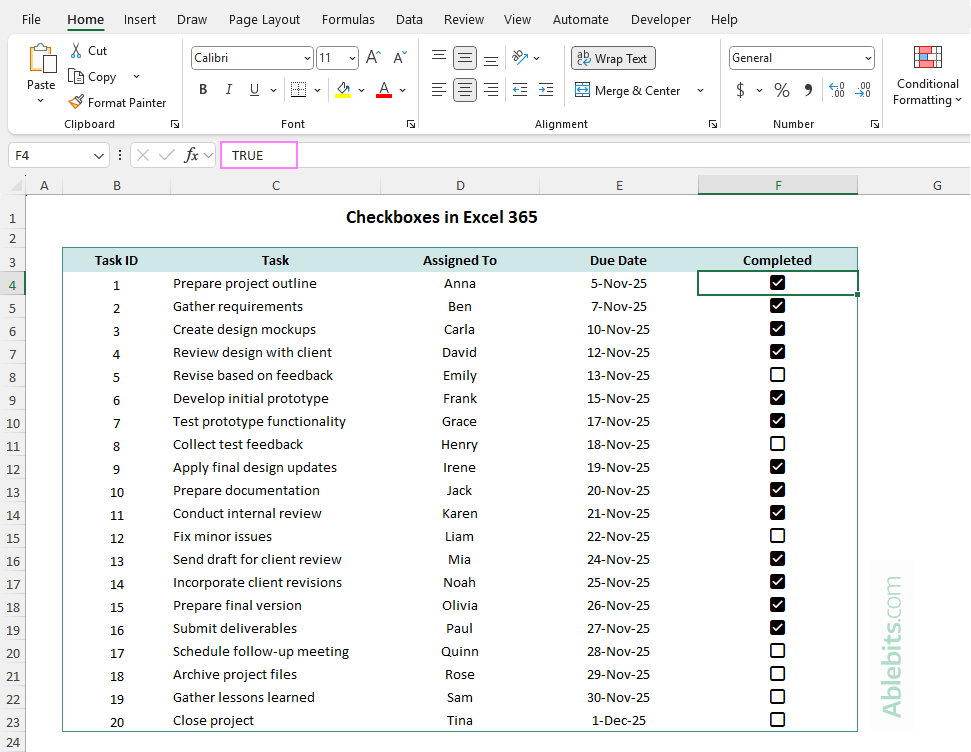
These native checkboxes are fully compatible with Excel formulas, conditional formatting, and dynamic arrays. They can be copied, moved, and filled down just like any other data in your sheets, making them far easier to use for interactive checklists and dashboards.
They work consistently across platforms, including Excel for Microsoft 365 (Windows and Mac) and Excel online.
How to insert a checkbox in Excel
Adding a checkbox in Excel 365 is very quick and straightforward. Here's how to insert it in just a couple of easy steps.
- Select one or more cells where you want to put a checkbox.
- On the Insert tab, in the Controls group, click the Checkbox button.
Done! Interactive checkboxes are added to all the selected cells at once:
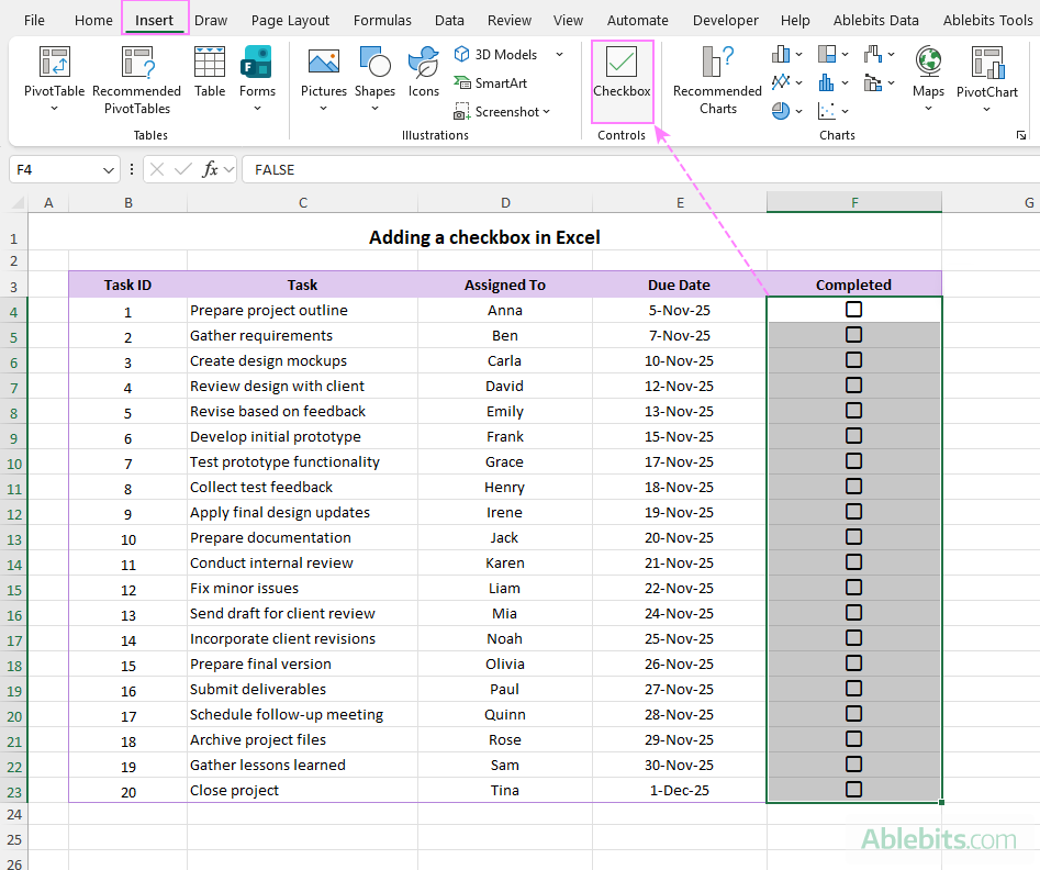
Tip. To put checkboxes in non-adjacent cells or ranges, hold down Ctrl while selecting each cell or range where you want a checkbox.
How to check or uncheck a checkbox in Excel
Once your checkboxes are added, you can easily mark items as done or clear them when needed.
There are two ways to toggle a checkbox in Excel:
- Using the mouse. Simply click the box once to check it and click again to uncheck it.
- With the Spacebar. Select the cell and press the Spacebar once to tick the checkbox. Then, press it again to remove the tick.
The second method is especially handy when you're navigating through your checklist with the arrow keys - perfect for those who like to work without lifting their hands from the keyboard.
How to tick multiple checkboxes in Excel
To check or uncheck several checkboxes at once:
- Select the range or individual cells containing the checkboxes.
- Press the Spacebar to check all the boxes.
- Press the Spacebar again to uncheck them all.
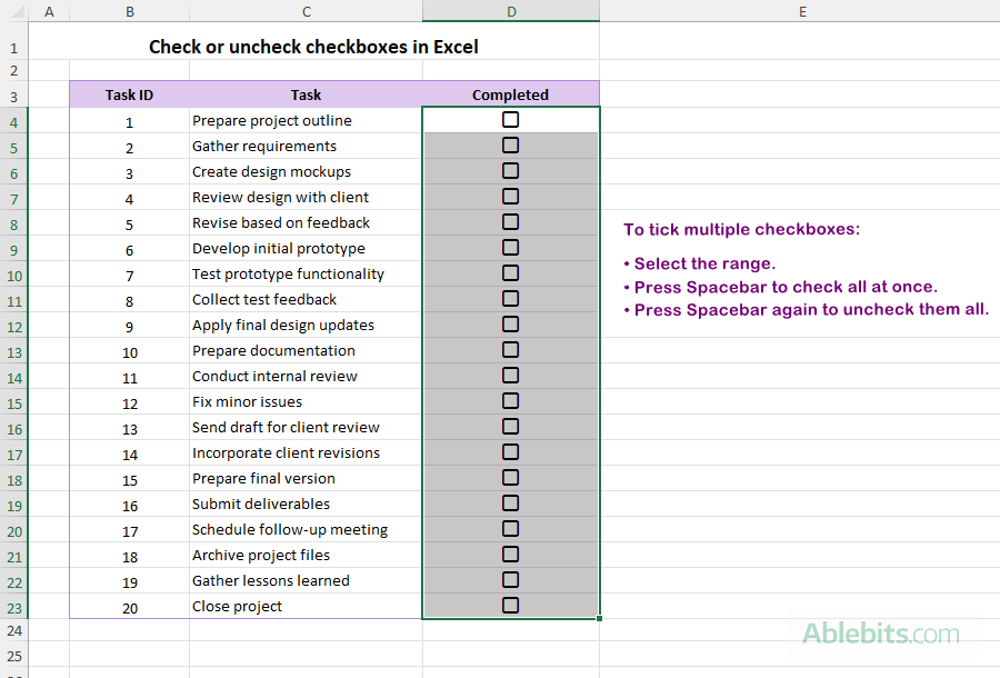
Keep in mind that the Spacebar behaves differently depending on the current state of the selected checkboxes:
- If some checkboxes in your selection are already checked, pressing the Spacebar once will clear all of them.
- Pressing the Spacebar again will check them all.
That's a quick and efficient way to manage Excel checklists with a couple of keystrokes, without reaching for the mouse.
How to delete checkbox in Excel
When you no longer need checkboxes in your worksheet, for example, after finishing a project or redesigning your layout, you can easily remove them.
- Select the cell or range of cells that contain the checkboxes you want to remove.
- Press Delete on your keyboard once or twice:
- If any of the selected checkboxes are checked, the first press of Delete will clear the tick marks but won't remove any checkboxes in the selected range. Press Delete a second time to remove them completely.
- If none of the selected boxes are checked, pressing Delete once will immediately remove all of them.
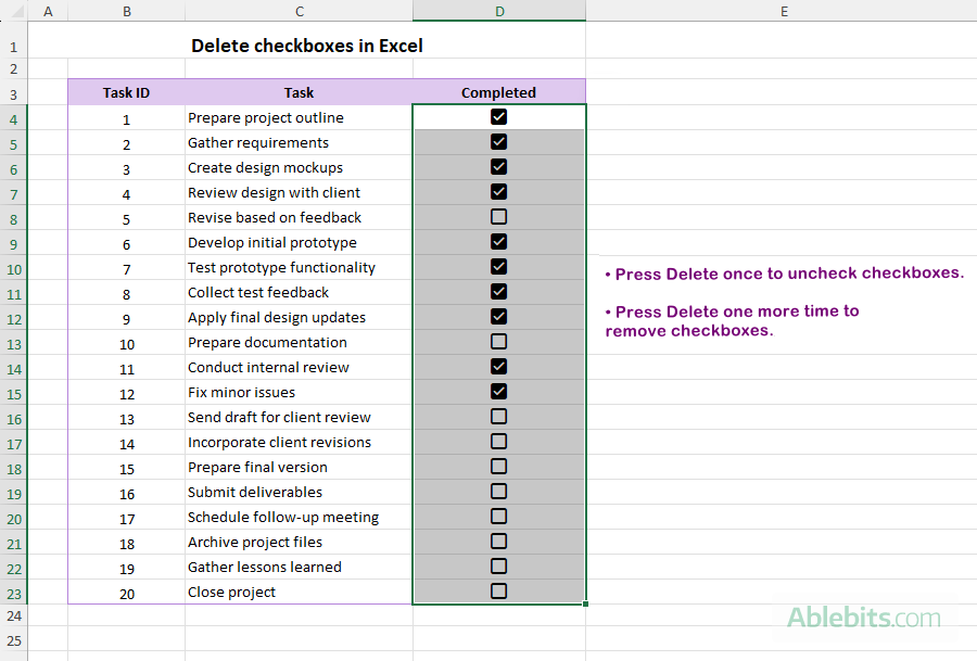
That's it! The checkbox is deleted, and its TRUE/FALSE value is cleared just like normal cell content.
Tip. If you've accidentally deleted a checkbox, press Ctrl + Z to undo the deletion and restore it.
How to strikethrough text when checkbox is checked in Excel
Turning an ordinary list into a checklist is one of the simplest yet most useful things you can do with checkboxes in your spreadsheets. And for an extra bit of clarity, you can have Excel automatically cross out each item when it's marked as done.
Here's how to strikethrough completed items with Excel conditional formatting:
- Select the cells you wish to format. In our case, to cross out only the task names in column C, select C4:C23. To strike through whole rows, select B4:E23.
- Go to the Home tab > Conditional Formatting > New Rule.
- Choose Use a formula to determine which cells to format.
- In the formula bar, enter a formula like the one below. Remember to adjust the reference to match your top-most checkbox.
=$F4=TRUE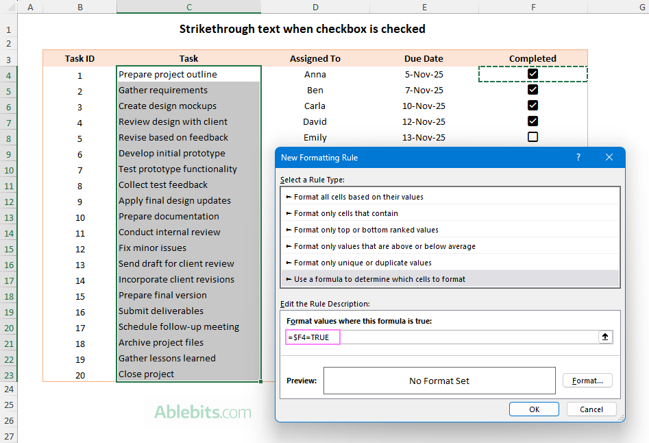
- Click Format, go to the Font tab, and select the Strikethrough effect.
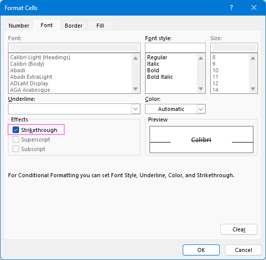
- Optionally, you can also choose a lighter font color to make completed tasks fade slightly into the background, making unchecked items stand out.
- Click OK to save the rule.
Now, when you check a box, the corresponding item will get automatically crossed out, giving you a visual cue of what's done and what's still pending.
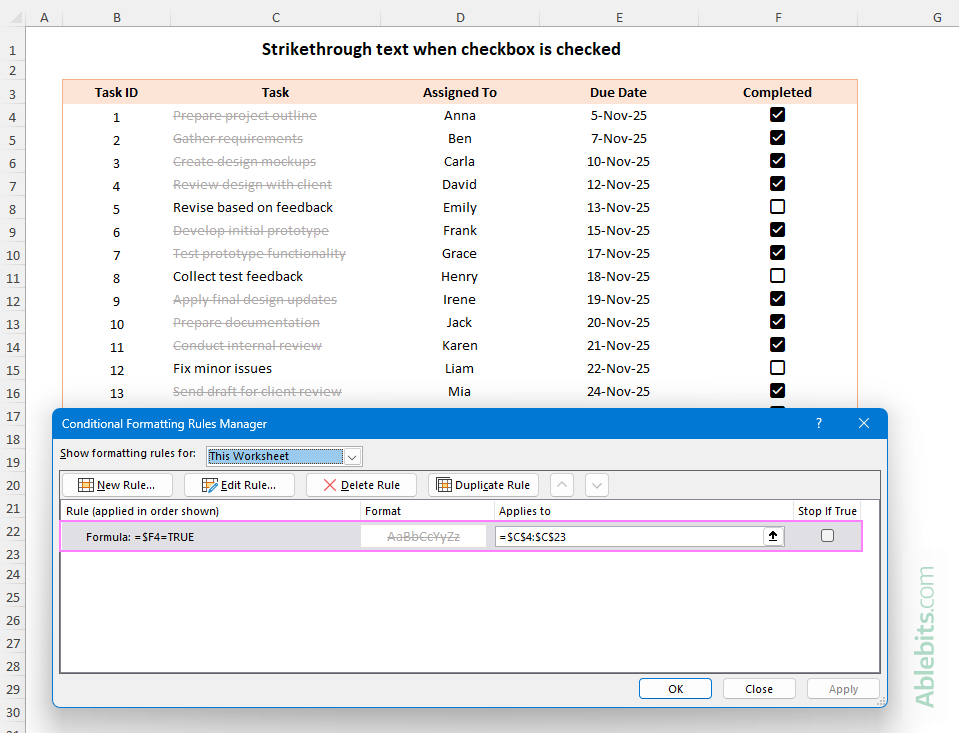
If you want to strikethrough entire rows instead of just one column, be sure to select the whole dataset except the checkbox column before creating the rule, or edit the existing rule so it applies to multiple columns – B4:E23 in the image below:
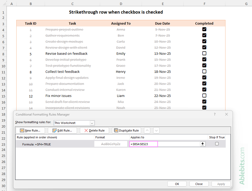
For more details, see How to set up conditional formatting rule based on formula.
Tip. In the formula, the dollar sign before the column letter ($F4) locks the column reference so it always points to column F, while the row reference remains relative. As a result, Excel checks the value in column F for each corresponding row. In this example, locking the column reference isn't mandatory, but it's helpful when you want to extend the same rule to other columns without adjusting the formula each time. For more information, please see Proper use of cell references in Excel conditional formatting.
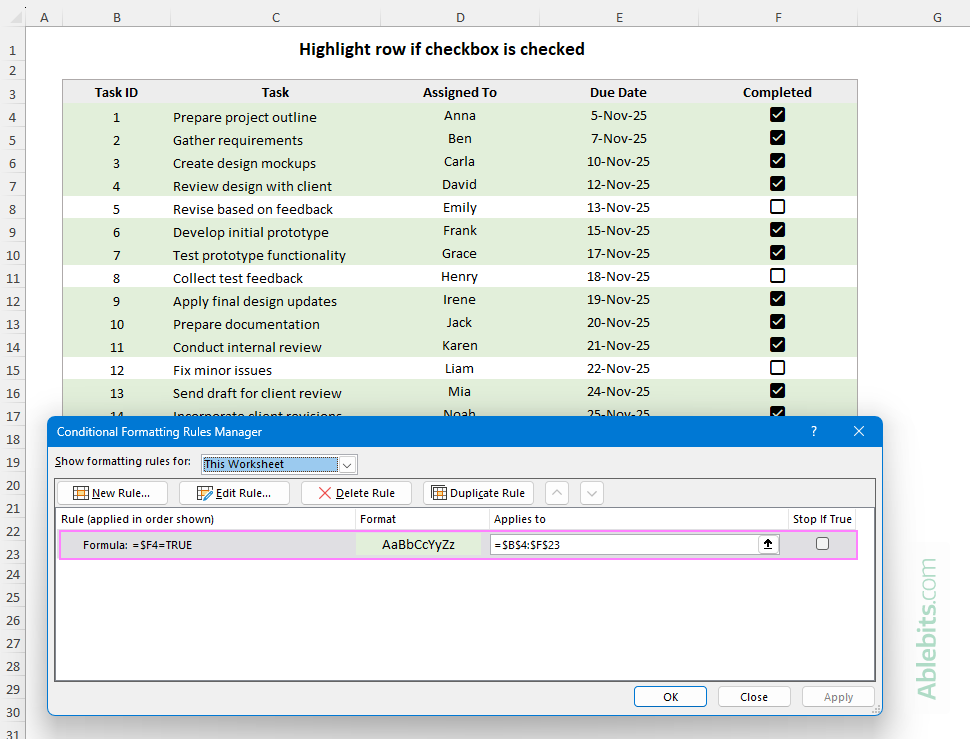
How to highlight row if checkbox is checked in Excel
Crossing out completed tasks is great, but seeing the whole row light up when you tick a checkbox may be even better.
With a conditional formatting rule, Excel can automatically highlight completed rows for you. Here's how to set it up:
- Select all the rows that contain your data (B4:F23 in this example).
- Head over to the Home tab > Conditional Formatting > New Rule > Use a formula to determine which cells to format.
- Enter a formula that refers to the top-most cell of the checkbox column. For example, if your checkboxes are in column F, starting in row 4:
=$F4=TRUE - Click Format and switch to the Fill tab.
- Pick a color to highlight completed rows (a light green works well).
- Click OK twice to close both windows and apply the rule.
Now, whenever you tick a checkbox, Excel will automatically highlight the entire row in the selected color.
Using a checkbox formula in Excel
Once your checkboxes are in place, you can use various formulas to summarize the results: count how many boxes are checked, how many remain unchecked, or calculate completion percentages. Since in Excel 365, checkboxes live directly inside cells and return TRUE (checked) or FALSE (unchecked), you can reference them in formulas just like regular Boolean values.
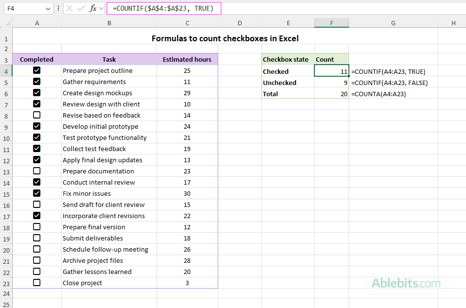
COUNTIF formula: Count checkboxes in Excel
You can count the total number of checkboxes, or specifically the checked and unchecked ones, using Excel's standard counting functions.
Count checked boxes
To count how many checkboxes are checked, use the COUNTIF function with the criteria argument set to TRUE, which is the logical value returned by a checked box.
Assuming the checkboxes are in the range A4:A23, the formula takes this form:
=COUNTIF(A4:A23, TRUE)
Count unchecked boxes
To find out how many boxes remain unchecked, apply the COUNTIF function with the criteria set to FALSE, the logical value of an unticked checkbox.
=COUNTIF(A4:A23, FALSE)
Count all checkboxes
To get the total number of checkboxes regardless of their state, use the COUNTA function that is designed for counting non-empty cells in the range. For example:
=COUNTA(A4:A23)
SUMIF formula: Sum if checkbox is ticked or not ticked
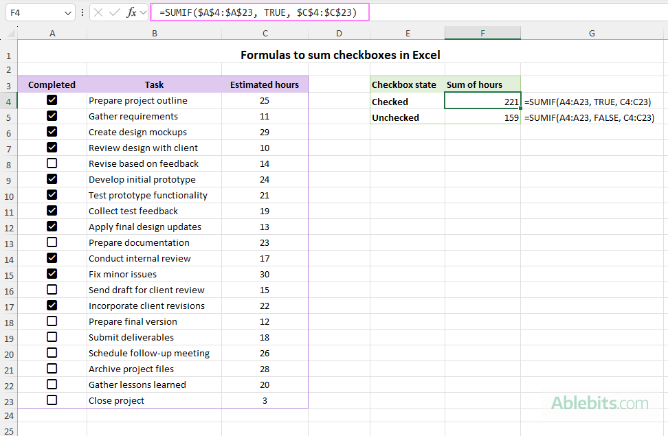
Checkboxes can do more than just show progress. You can also use them to sum related values automatically. This can be done with the help of the SUMIF function, which adds up numbers only when a certain condition is met.
Sum if checkbox is checked
To total the values for checked boxes, use SUMIF with the condition set to TRUE.
In the dataset below, to sum estimated hours for tasks that are marked as completed, the formula is:
=SUMIF(A4:A23, TRUE, C4:C23)
Sum if checkbox is unchecked
To total hours for tasks that haven't been ticked off yet, change the condition to FALSE.
=SUMIF(A4:A23, FALSE, C4:C23)
Where A4:A23 is the range with checkboxes and C4:C23 are the numeric values to add up.
Calculate percentage of checkboxes in Excel
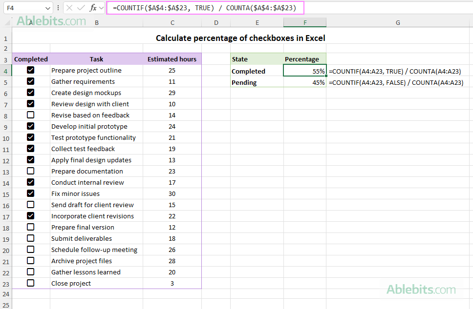
To show overall progress as a percentage (in other words, how much of your checklist is complete), you can use Excel's classic percentage formula, where you simply divide part by total.
To calculate the percentage of checked boxes, use the formula that divides the number of checked boxes (TRUE) by the total number of boxes in the range:
=COUNTIF(A4:A23, TRUE) / COUNTA(A4:A23)
To find the percentage of unchecked boxes, utilize a similar formula:
=COUNTIF(A4:A23, FALSE) / COUNTA(A4:A23)
Format the result as percentage, and you'll get a completion rate like shown in the screenshot below:
Tip. Combine these formulas with a progress bar to create a simple dashboard that updates automatically as you check off tasks.
If checkbox is checked then formula
You can perform almost any calculation in Excel based on checkbox values. As each checkbox returns TRUE when it's checked and FALSE when it's not, you can reference its cell within the IF function to perform different calculations or show different outputs depending on the checkbox state.
Display certain text when checkbox is checked
To show a simple message such as Done / Pending or Yes /No, you can use a basic IF formula like this:
=IF(C4=TRUE, "Yes", "No")
It evaluates whether the checkbox in cell B4 is ticked. If it is, the formula returns "Yes", otherwise, "No".
Alternatively, you can mark an item as "Done" when a box is checked and leave it blank when it's not:
=IF(C4=TRUE, "Done", "")
Perform calculation if checkbox is ticked
You can also perform various numeric calculations based on checkbox values. For instance, you can increase the value in a related cell by certain percentage if the box is checked - handy for applying bonuses or discounts.
In this example, we enter the below formula in cell E4 to increase the amount in B4 by 10% if the box in C4 is checked, i.e. if the bonus is applied:
=IF(C4=TRUE, B4*(1+10%), B4)
Or simply:
=IF(C4=TRUE, B4*1.1, B4)
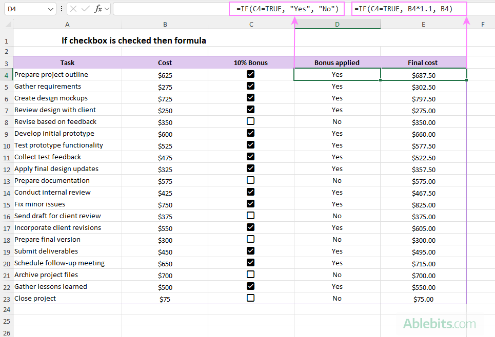
Tip. In the above formulas, we use C4=TRUE as the logical test. In theory, you can simply reference the cell itself, and the shorter version =IF(C4, "Yes", "No") will work the same way. However, it's considered good practice to state the logical condition explicitly for clarity.
How to filter checkboxes in Excel
When your dataset includes checkboxes, it can be helpful to quickly view only the rows that are ticked or not. In Excel 365, there are a few easy ways to filter data by checkbox state.
Filter checkboxes using Excel AutoFilter
The simplest and most obvious way to filter your data based on checkboxes is to use Excels built-in AutoFilter.
- Select any cell in your dataset.
- On the Home tab, in the Editing group, click Sort & Filter > Filter.
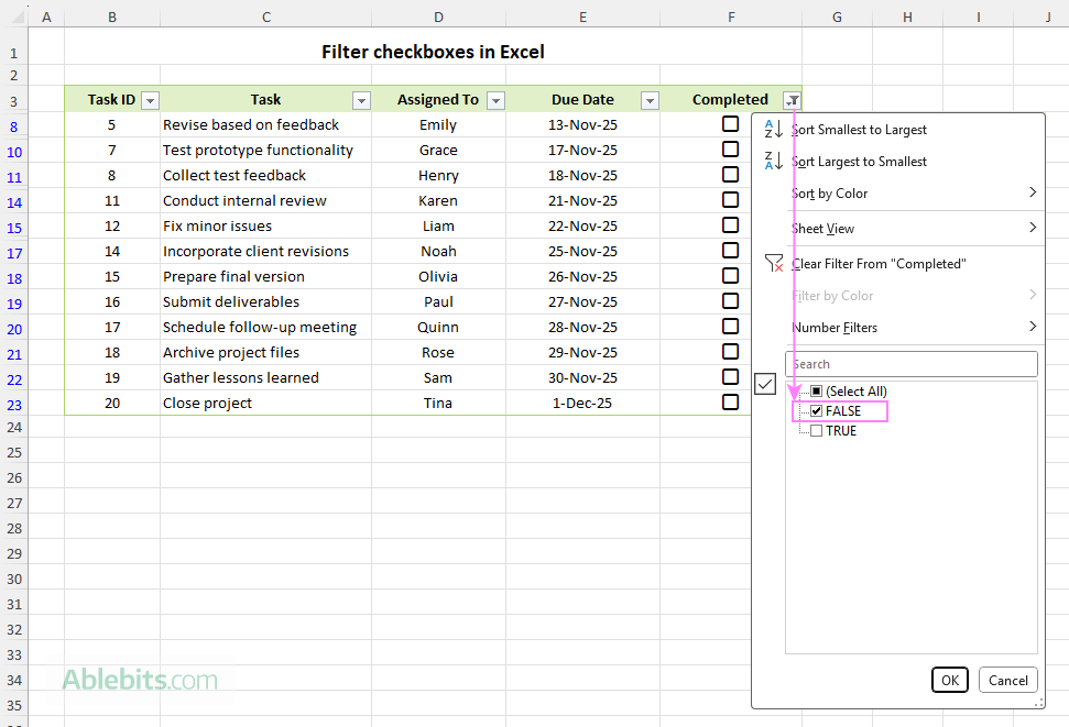
- Click the drop-down filter arrow in the column containing checkboxes.
- Check TRUE to show the ticked boxes or FALSE to show the unticked ones.
This method works well for both regular ranges and Excel tables (which include column filters by default).
Filter by checkbox dynamically with formula
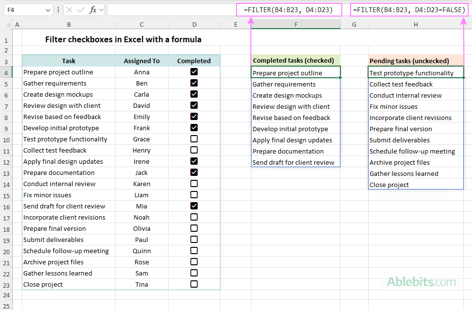
If you want a dynamic view that updates automatically, use the FILTER function.
To display only checked rows:
=FILTER(B4:B23, D4:D23=TRUE)
Or
=FILTER(B4:B23, D4:D23)
To show only unchecked rows:
=FILTER(B4:B23, D4:D23=FALSE)
Where B4:B23 are the task names to return and D4:D23 are the checkboxes.
This approach is particularly effective for dashboards and summaries, since you can choose exactly which columns to include in the FILTER output. The results update automatically in real time whenever checkboxes are ticked or cleared.
Filter checkboxes with a slicer
If your data is formatted as an Excel Table, you can add a slicer to filter by checkbox values interactively.
- Conver your data range to a table using the Ctrl + T shortcut.
- On the Insert tab, in the Filters group, click Slicer.
- In the Insert Slicers dialog box, select the column where your checkboxes are located, and click OK.
Now, you can use the slicer buttons (TRUE and FALSE) to filter the table based on checkboxes with a single click.
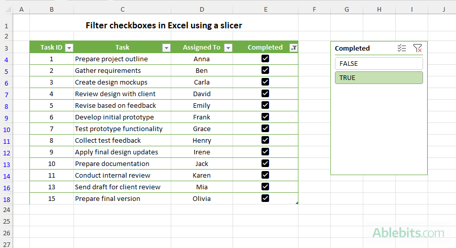
Slicers are very handy when sharing or presenting data, as they make filtering visual and easy for anyone to use.
For more information, see Create slicer for Excel table.
Make a progress tracker with checkboxes in Excel
With the help of checkboxes, you can easily create a progress tracker that shows how far along each project is and what's still left to do.
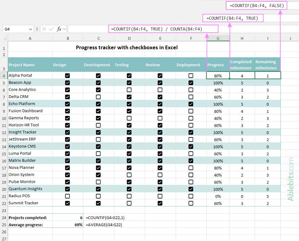
As an example, we are going to use the Project Milestone Tracker dataset, which contains project names in column A and five milestone columns (B to F). Each milestone cell contains a checkbox (please see the image below).
Calculate progress percentage
In F4, enter the following formula and copy it down the column:
=COUNTIF(B4:F4, TRUE) / COUNTA(B4:F4)
This formula counts how many milestones in the current row are checked (TRUE) and divides that by the total number of milestone columns. Format the Progress column as a percentage, and you'll instantly see how complete each project is.
Count complete and remaining milestones
To show how many milestones are done or still pending, use the following formulas.
In H4, count the number of completed milestones per project:
=COUNTIF(B4:F4, TRUE)
In E4, count how many milestones are still unchecked, showing how many steps remain:
=COUNTIF(C4:G4, FALSE)
Fill both formulas down the column to calculate values for all projects.
Add summary section
For a quick overview, you can create a summary at the top or bottom of your sheet with formulas like these.
Projects completed:
=COUNTIF(G4:G22,1)
Average progress:
=AVERAGE(G4:G22)
Highlight completed projects
To make finished projects stand out, apply conditional formatting to highlight rows where progress equals 100%. Use either of the following formulas:
=$G4=1
=COUNTIF($B2:$F2, TRUE)=5
The first formula checks whether the value in the Progress column (G) equals 1 (i.e. 100%), while the second one verifies if all five milestones are checked. Both methods work the same, highlighting every row where the project is fully complete, so you can spot them at a glance.
Tip. Once your Excel progress tracker is ready, the next step might be adding a progress bar that fills automatically as tasks are marked are completed.
How native checkboxes behave in Excel
Below are a few interesting facts about checkboxes in Excel 365 that may not be obvious at first glance. Understanding these small nuances can help you use them more effectively, especially when working with formulas or logical values.
- Default state. When you insert a new checkbox, it is unchecked by default, and the cell value is FALSE. Once you tick it, the value changes to TRUE.
- Deleting checkboxes. When you delete checkboxes from cells, their underlying TRUE and FALSE values are also removed.
- Removing boxes but keeping logical values. If you want to remove the visible checkboxes but keep their current Boolean values, select the cells, then go to the Home tab > Clear > Clear Formats. The checkboxes will disappear, but the TRUE/FALSE results will remain in cells.
- Checkboxes and logical values. If your cells already contain TRUE or FALSE values (typed directly or returned by formulas), Excel allows you to insert checkboxes in the same cells. However, they will behave differently:
- Checkboxes placed on top of constant logical values behave normally - you can click them to check or uncheck.
- Checkboxes placed over formulas that return TRUE or FALSE are read-only. You can't manually change their state; only the formula's result can toggle the checkbox.
Excel 365 checkbox missing
If you don't see the Checkbox option in the Insert tab, there are a couple of possible reasons:
- Your Excel version doesn't support it. Native in-cell checkboxes are available only in Excel 365 (Windows, Mac, and Web). Older versions such as Excel 2021, 2019, or 2016 still require using Form Controls instead.
- Your Excel needs an update. If you have a Microsoft 365 subscription, make sure your Excel app is updated to the latest version. To check for updates, go to File > Account > Update Options > Update Now (on Windows) or Help > Check for Updates (on Mac).
That's how to add and use modern checkboxes in Excel. With the techniques you've learned, you can build elegant, interactive sheets that respond instantly to the user input and are both functional and pleasant to work with.
Practice workbook for download
Using checkboxes in formulas (.xlsx file)
 by
by