The tutorial explains what the Compound Annual Growth Rate is, and how to make a clear and easy-to-understand CAGR formula in Excel.
In one of our previous articles, we unveiled the power of compound interest and how to calculate it in Excel. Today, we'll take a step further and explore different ways to compute Compound Annual Growth Rate (CAGR).
In simple terms, CAGR measures the return on an investment over a certain period of time. Strictly speaking, it's not an accounting term, but it is often used by financial analysts, investment managers and business owners to figure out how their business has developed or compare revenue growth of competing companies.
In this tutorial, we won't be digging deeply in arithmetic, and focus on how to write an effective CAGR formula in Excel that allows calculating compound annual growth rate based on 3 primary input values: investment's beginning value, ending value, and time period.
What is Compound Annual Growth Rate?
Compound Annual Growth Rate (CAGR for short) is a financial term that measures the mean annual growth rate of an investment over a given period of time.
To better understand the CAGR logic, let's have a look at the following example. Supposing, you see the below numbers in a financial report of your company:

It's no big deal to calculate a year-to-year growth rate using a regular percentage increase formula like shown in the screenshot below:

But how do you get a single number that shows a growth rate over 5 years? There are two ways to compute this - Average and Compound annual growth rate. The compound growth rate is a better measure because of the following reasons:
- Average annual growth rate (AAGR) is the arithmetic mean of a series of growth rates, and it is easily calculated using a normal AVERAGE formula. However, it totally ignores the compounding effects and therefore the growth of an investment can be overestimated.
- Compound annual growth rate (CAGR) is a geometric average that represents the rate of return for an investment as if it had compounded at a steady rate each year. In other words, CAGR is a "smoothed" growth rate that, if compounded annually, would be equivalent to what your investment achieved over a specified period of time.
CAGR formula
The generic CAGR formula used in business, finance and investment analysis is as follows:

Where:
- BV - Beginning value of the investment
- EV - Ending value of the investment
- n - Number of periods (like years, quarters, months, days, etc.)
As demonstrated in the following screenshot, the Average and CAGR formulas return different results:

To make things easier to understand, the following image shows how CAGR is calculated for different periods in terms of BV, EV, and n:

How to calculate CAGR in Excel
Now that you have a basic idea of what Compound Annual Growth Rate is, let's see how you can calculate it in your Excel worksheets. Overall, there are 4 ways to create an Excel formula for CAGR.
Formula 1: Direct way to create a CAGR calculator in Excel
Knowing the generic CAGR formula discussed above, creating a CAGR calculator in Excel is a matter of minutes, if not seconds. Just specify the following values in your worksheet:
- BV - Beginning value of the investment
- EV - Ending value of the investment
- n - Number of periods
And then, enter the CAGR formula in an empty cell:
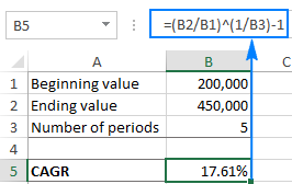
In this example, BV is in cell B1, EV in B2, and n in B3. So, we enter the following formula in B5:
=(B2/B1)^(1/B3)-1

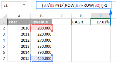
If you have all investment values listed in some column, then you can add a degree of flexibility to your CAGR formula and have it calculate the number of periods automatically.
To calculate CAGR in our sample worksheet, the formula is as follows:
=(B7/B2)^(1/(ROW(B7)-ROW(B2)))-1

Tip. If the output value displays as a decimal number, apply the Percentage format to the formula cell.
CAGR formula 2: RRI function
The easiest way to calculate Compound Annual Growth Rate in Excel is by using the RRI function, which is designed to return an equivalent interest rate on a loan or investment over a specific period based on the present value, future value and the total number of periods:
Where:
- Nper is the total number of periods.
- Pv is the present value of the investment.
- Fv is the future value of the investment.
With nper in B4, pv in B2 and fv in B3, the formula takes this form:
=RRI(B4, B2, B3)

CAGR formula 3: POWER function
Another quick and straightforward way to calculate CAGR in Excel is by using the POWER function that returns the result of a number raised to a certain power.
The syntax of the POWER function is as follows:
Where number is the base number, and power is the exponent to raise the base number to.
To make an Excel CAGR calculator based on the POWER function, define the arguments in this way:
- Number - ending value (EV) / beginning value (BV)
- Power - 1/number of periods (n)
And here is our POWERful CAGR formula in action:
=POWER(B7/B2,1/5)-1

Like in the first example, you can have the ROW function to calculate the number of periods for you:
=POWER(B7/B2,1/(ROW(B7)-ROW(B2)))-1
CAGR formula 4: RATE function
One more method for calculating CAGR in Excel is using the RATE function that returns the interest rate per period of an annuity.
At first sight, the syntax of the RATE function looks a bit complicated, but once you understand the arguments, you may like this way to calculate CAGR in Excel.
- Nper - the total number of payments for the annuity, i.e. the number of periods over which a loan or investment should be paid. Required.
- Pmt - the amount of the payment made each period. If omitted, the fv argument must be supplied.
- Pv - the present value of the investment. Required.
- Fv - the future value of the investment at the end of nper payments. If omitted, the formula takes on the default value of 0.
- Type - an optional value that indicates when payments are due:
- 0 (default) - payments are due at the end of the period.
- 1 - payments are due at the beginning of the period.
- Guess - your guess for what the rate might be. If omitted, it is assumed to be 10%.
To turn the RATE function into a CAGR calculation formula, you need to supply the 1st (nper), 3rd (pv) and 4th (fv) arguments in this way:
I will remind you that:
- BV is the beginning value of the investment
- EV is the ending value of the investment
- n is the number of periods
Note. Be sure to specify the beginning value (BV) as a negative number, otherwise your CAGR formula would return a #NUM! error.
To calculate the compound growth rate in this example, the formula is as follows:
=RATE(5,,-B2,B7)
To spare yourself the trouble of calculating the number of periods manually, you can have the ROW function compute it for you:
=RATE(ROW(B7)-ROW(B2),,-B2,B7)

CAGR formula 5: IRR function
The IRR function in Excel returns the internal rate of return for a series of cash flows that occur at regular time intervals (i.e. days, months, quarters, years, etc.). It has the following syntax:
Where:
- Values - a range of numbers that represent the cash flows. The range must contain at least one negative and at least one positive value.
- [Guess] - an optional argument that represents your guess at what the rate of return might be. If omitted, the default value of 10% is taken.
Because the Excel IRR function is not exactly designed for calculating compound growth rate, you would have to reshape the original data in this way:
- The beginning value of investment should be entered as a negative number.
- The ending value of investment is a positive number.
- All intermediate values are zeros.

Once your source data is reorganized, you can calculate CAGR with this simple formula:
=IRR(B2:B7)
Where B2 is the beginning value and B7 is the ending value of investment:

Well, this is how you can calculate CAGR in Excel. If you have been following the examples closely, you might have noticed that all 4 formulas return the identical result - 17.61%. To better understand and probably reverse-engineer the formulas, you are welcome to download the sample worksheet below. I thank you for reading and hope to see you on our blog next week!
Practice workbook for download
CAGR Calculation Formulas (.xlsx file)
 by
by
11 comments
What if I need to know my ending value? CAGR is at 3%, 5yrs, and my beginning value is 20,000. How do I compute the ending value?
FV function should get you the desired output
CAGR for period less than a year, for example 5 months and 17 days, can i have the formula please
for months or days, this formula always helps me to calculate the rate between two-quarters of revenue = rate(1,(initial value),(final value)
Thank you for the amazing explanation
But How to calculate annualised return if the stock or asset is held for less than a year, let's say Stock is held for a few months but We would like to calculate its annualised return?
In that case, you can still annualize the return. Consider the following example.
You got 6% return on a share with holding period of 6 months. you can annualize return by 6%*12/6 = 12%.
Why such a complicated step to calculate CAGR.. when Excel has RRI function.
So the formula will be:
=RRI(No. of Years, Starting Amount, Ending Amount), This returns CAGR % over the years.
very simple and beautiful. All other formulas are NOT intuitive for normal user.
Note: the RRI function has three arguments (number of years = 5, start = 100, end = 147).
Hi Fiaz,
It is indeed a very simple and elegant solution. I have added the RRI formula to our tutorial. Thank you for the tip!
In my experience you should never use fixed numbers in your formulas because it leeds to simple mistakes...
For example in the power formula you should use:
=POWER(B7/B2;1/COUNT(B2:B7))-1
and the result is 14.47% because in the formula you use 5 years but your data isfor 6
Hello Rado,
Thank you for your comment. Right, the data is for 6 years, which makes 5 periods. Therefore, instead of COUNT, you'd better use the ROW function to calculate the number of periods:
=POWER(B7/B2,1/(ROW(B7)-ROW(B2)))-1
The result will be 17.61% like in all other formulas.
i didnt see that n stands for periods sorry :D