This short tutorial shows how to copy formatting in Excel using Format Painter, Fill Handle and Paste Special options. These techniques work in all versions of Excel, from 2007 through Excel 365.
After you've put a lot of effort in calculating a worksheet, you would usually want to add some finishing touches to make it look nice and presentable. Whether you are creating a repot for your head office or building a summary worksheet for the board of directors, proper formatting is what makes important data stand out and convey the relevant information more effectively.
Fortunately, Microsoft Excel has an amazingly simple way to copy formatting, which is often overlooked or underestimated. As you have probably guessed, I am talking about the Excel Format Painter that makes it really easy to take the formatting of one cell and apply it to another.
Further on in this tutorial, you will find the most efficient ways to use Format Painter in Excel, and learn a couple of other techniques to copy formatting in your sheets.
Excel Format Painter
When it comes to copying formatting in Excel, Format Painter is one of the most helpful and underused features. It works by copying the formatting of one cell and applying it to other cells.
With just a couple of clicks, it can help you reproduce most, if not all of the formatting settings, including:
- Number format (General, Percentage, Currency, etc.)
- Font face, size, and color
- Font characteristics such as bold, italic, and underline
- Fill color (cell background color)
- Text alignment, direction and orientation
- Cell borders
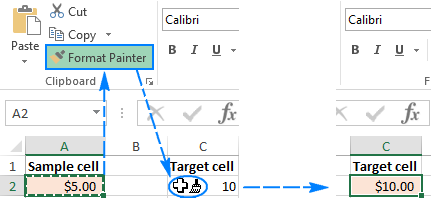
In all Excel versions, the Format Painter button is located on the Home tab, in the Clipboard group, right next to the Paste button:

How to use Format Painter in Excel
To copy cell formatting with the Excel Format Painter, just do the following:
- Select the cell with the formatting you want to copy.
- On the Home tab, in the Clipboard group, click the Format Painter button. The pointer will change to a paint brush.
- Move to the cell where you want to apply the formatting and click on it.
Done! The new formatting is copied to your target cell.

Excel Format Painter tips
If you need to change formatting of more than one cell, clicking each cell individually would be tedious and time consuming. The following tips will speed things up.
1. How to copy formatting to a range of cells.
To copy formatting to several adjacent cells, select the sample cell with the desired format, click the Format Painter button, and then drag the brush cursor across the cells that you want to format.

2. How to copy format to non-adjacent cells.
To copy formatting to non-contiguous cells, double-click the Format Painter button instead of single-clicking it. This will "lock" the Excel Format Painter on, and the copied formatting will be applied to all cells and ranges that you click/select until you press Esc or click on the Format Painter button one final time.
3. How to copy the formatting of one column to another column row-by-row
To quickly copy the format of the entire column, select the heading of the column whose formatting you want to copy, click Format Painter, and then click the heading of the target column.
As demonstrated in the following screenshot, the new formatting is applied to the target column row-by-row, including the column width:

In a similar manner, you can copy the format of the entire row, column-by-column. For this, click the sample row heading, click Format Painter, and then click the heading of the target row.
As you have just seen, the Format Painter makes copying format as easy as it can possibly be. However, as is often the case with Microsoft Excel, there is more than one way to do the same thing. Below, you will find two more methods to copy formats in Excel.
How to copy formatting down a column using the Fill Handle
We often use the fill handle to copy formulas or auto fill cells with data. But did you know that it can also copy Excel formats with just a few clicks? Here's how:
- Format the first cell the way you want.
- Select the properly formatted cell and hover over the fill handle (a small square at the lower right-hand corner). As you do this, the cursor will change from the white selection cross to a black cross.
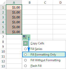
- Hold and drag the handle over the cells where you want to apply the formatting:

This will also copy the value of the first cell to other cells, but don't worry about that, we will undo it on the next step. - Release the fill handle, click the Auto Fill Options drop-down menu, and select Fill Formatting Only:

That's it! The cell values revert to the original values, and the desired format is applied to other cells in the column:

Tip. To copy the formatting down the column until the first empty cell, double-click the fill handle instead of dragging it, then click AutoFill Options, and select Fill Formatting Only.
How to copy cell formatting to an entire column or row
Excel Format Painter and Fill Handle work great with small selections. But how do you copy the format of a specific cell to an entire column or row so that the new format is applied to absolutely all cells in a column/row including blank cells? The solution is using the Formats option of Excel Paste Special.
- Select the cell with the desired format and press Ctrl+C to copy its content and formats.
- Select the entire column or row that you want to format by clicking on its heading.
- Right-click the selection, and then click Paste Special.
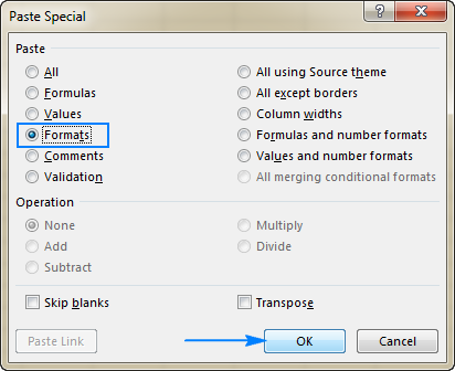
- In the Paste Special dialog box, click Formats, and then click OK.

Alternatively, select the Formatting option from the Paste Special pop-up menu. This will display a live preview of the new format, as shown in the screenshot below:

Shortcuts to copy formatting in Excel
Regrettably, Microsoft Excel doesn't provide a single shortcut that you could use to copy cell formats. However, this can be done by using a sequence of shortcuts. So, if you prefer working form the keyboard most of the time, you can copy format in Excel in one of the following ways.
Excel Format Painter shortcut
Instead of clicking the Format Painter button on the ribbon, do the following:
- Select the cell containing the required format.
- Press Alt, H, F, P keys.
- Click the target cell where you want to apply the formatting.
Please note, the shortcut keys for Format Painter in Excel should be pressed one by one, not all at once:
- Alt activates the keyboard shortcuts for ribbon commands.
- H selects the Home tab on the ribbon.
- F, P select the Format Painter button.
Paste Special formatting shortcut
Another quick way to copy format in Excel is by using the keyboard shortcut for Paste Special > Formats:
- Select the cell from which you want to copy the format.
- Press Ctrl + C to copy the selected cell to the Clipboard.
- Select the cell(s) to which the format should be applied.
- Press Shift + F10, R and then click Enter.
This key sequence does the following:
- Shift + F10 displays the context menu.
- Shift + R chooses to paste only formatting.
These are the fastest ways to copy formatting in Excel. If you've accidentally copied a wrong format, no problem, our next article will teach you how to clear it :) I thank you for reading and hope to see you on our blog soon!
 by
by
19 comments
Explanation is very good
Do you know of a way to copy just the color versus the full cell format? Kind of a pain to have to open the fill color, find the RGB or hex to set the cell fill color the same. Tks.
Hi! Unfortunately Excel only allows you to copy the entire cell format. I think you can copy only the color by using the VBA macro.
The shortcut for Paste Formats is now shorter: Shift+F10 R
Thank you, Rodolfo! Updated the info in the article.
I would like to copy the data in row 1 and insert this to all the data below .
how to do it? Thank you
Hi! Maybe this article will be helpful: Excel Paste Special: copy values, comments, column's width and more.
Hi, I have a filter formula, whereby I am only displaying one row of data at a time on a separate sheet based on the filter selected. Example(=FILTER(B5:D14,D5:D14=H2,"No results")
The cells in b5:d14 have a conditional formatting on them to highlight in colour.
How do I pull across the colours to the filtered cells?
Hi!
The FILTER function extracts only values from the table, not formatting. You can create new conditional formatting rules in the cells of the FILTER function.
I would like to create a HotKey to allow copying of a the complete cell format to another cell or groups of cells. Having to "hit" Alt-H-F-P is too many keys. I want to set up a hotkey so that I can simply press Ctrl + (A single key) to copy the complete format of that cell.
I am using Office Professional 2016.
Is it possible to create a HotKey?
Use quick access toolbar and add format painter, then you can get an Alt + number combination
I would like to copy the conditional formatting from one row to another.......I have tried "Paste Special", but this still requires a LOT of editing. (my worksheet will have about 800 row, and I wish to apply the same formula to each row)
RULE
Formula: =$E$4="Open" Format (Red colour) Applied to: =$B4:$J$4
If I use "Paste Special", every row is dependant upon $E$4
Formula: =$E$4="Open" Format (Red colour) Applied to: =$B25:$J$25
Formula: =$E$4="Open" Format (Red colour) Applied to: =$B26:$J$26
Formula: =$E$4="Open" Format (Red colour) Applied to: =$B27:$J$27
Formula: =$E$4="Open" Format (Red colour) Applied to: =$B28:$J$28
What I want is the formatting to be dependant upon its own row.
Formula: =$E$25="Open" Format (Red colour) Applied to: =$B25:$J$25
Formula: =$E$26="Open" Format (Red colour) Applied to: =$B26:$J$26
Formula: =$E$27="Open" Format (Red colour) Applied to: =$B27:$J$27
Formula: =$E$28="Open" Format (Red colour) Applied to: =$B28:$J$28
Hello!
I recommend copying the conditional formatting. However, do not use absolute references in condition formulas.
These instructions do not work. What about 365?
Hi,
Please describe your problem in more detail. It’ll help me understand it better and find a solution for you. Thank you.
I would like to copy the value of one cell and its font and shaded color by simply using the =A2 formula.
Cell A2 might be italicized and shaded yellow; if it is, then I need the other cell to reflect that formatting automatically.
How is this accomplished?
This should work:
Select the cell you like the look of and then click Format Painter, and then click the cell you want to format. Just using =A2 won't copy the formatting.
Hi, I'm familiar with the Format Painter, but my corporate laptop was just upgraded to Office 2016 (from 2011 for Mac). In Excel, when using the Format Painter, it will sometimes not apply the same font or color as the original. Sometimes it will. Any idea what is up?
Just a suggestion, but check the formatting of your destination cell. Clear any and all existing formatting. And check for any conditional formatting.
That is, if after six years you haven't found a solution.
?
But this might be helpful to others.