In this guide, you'll learn how to create different types of progress bars in Excel to track your projects, goals, or milestones. We'll start with conditional formatting data bars in cells, move on to professional bar charts, and finish with a circular version that looks great on any dashboard.
If you've already used Excel checkboxes to track project milestones, a progress bar is the perfect next step. It gives you a clear visual snapshot of how close you are to reaching a goal. In Excel, you can easily create a progress bar using conditional formatting or charts, no coding required. Let's walk through how to set it up step by step.
How to make a progress bar in Excel cell
A great way to make your project tracker more visual is to show a progress bar with percentage directly in a cell. Each time you check off a task, the bar will update dynamically showing how far along the project is.
Step 1. Insert checkboxes
When your goal is to track specific milestones or tasks within a project, checkboxes are a simple and effective tool. Each box represents an item that can be marked as complete or left unchecked until it's done.
The way you insert checkboxes depends on your Excel version:
- Excel 2021 – 2013: Insert a Check Box Form control or ActiveX control.
- Excel 365: Add native checkboxes via the View tab > Controls group > Checkbox button.
Step 2. Link checkboxes to cells (for Form Controls only)
If you added Form Control checkboxes, be sure to link each one to a cell, so Excel can record its status. Checked boxes return TRUE, while unchecked ones return FALSE, and these are the key values for calculating completion percentage.
The TRUE/FALSE values in linked cells can clutter your sheet, so it's best to hide those cells. Or you can use this smart trick to make the values invisible while keeping them fully-functional:
- Link each checkbox to the same cell where it resides. For this, right-click the checkbox, select Format Control, switch to the Control tab, and enter the reference in the Cell link box.
- Select all linked cells and press Ctrl + 1 to open the Format Cells dialog box.
- On the Number tab, select Custom, and enter ;;; (3 semicolons) in the Type box.
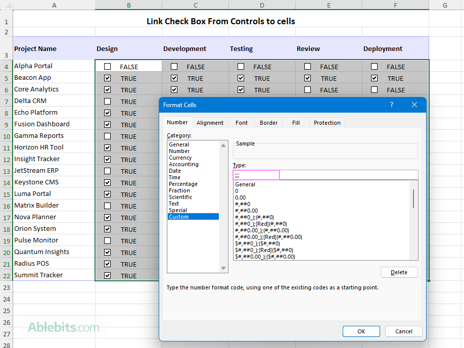
This custom number format hides any content in those cells, so TRUE and FALSE values won't appear on the worksheet but will still show up in the formula bar.
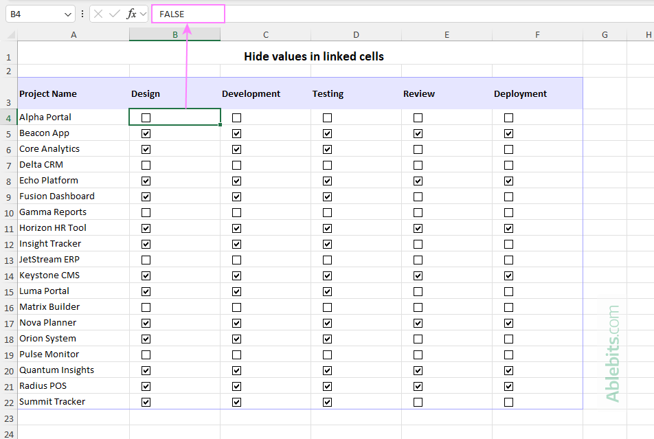
Note. In-cell Excel 365 checkboxes automatically return TRUE/FALSE values to their cells, so simply skip this step if you use them.
Step 3. Calculate completion percentage
Next, we'll use a simple formula to calculate how much of each project is complete:
Use the COUNTIF function to get the number of checked boxes (TRUE values), and COUNTA to count the total boxes in a row. Divide the first by the second to get a completion percentage.
For example, if your project milestones are in columns B to F, and data starts in row 4, enter this formula in G4 and copy it down to the remaining rows:
=COUNTIF(B4:F4, TRUE) / COUNTA(B4:F4)
Format the resulting values as percent. Each row will now show a dynamic completion percentage that updates automatically as you tick off boxes.

Step 4. Add Conditional Formatting Data Bars
Now it's time to turn those percentages into progress bars:
- Select the cells with your progress values (G4:G22 in our case).
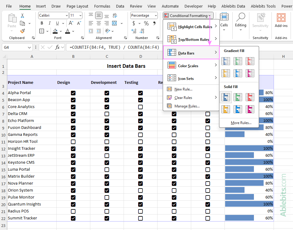
- On the Home tab, click Conditional Formatting > Data Bars.
- Choose a style you like: solid fill or gradient fill.
You'll immediately see colored bars filling each cell proportionally to its percentage value - 100% fills the cell completely, while 50% fills halfway. If your bars display progress incorrectly at this point, do not worry, the next step will fix it.
Step 5. Customize data bars
To make your progress bars work correctly and look nicer, go to Conditional Formatting > Manage Rules > Edit Rule and adjust the following options:
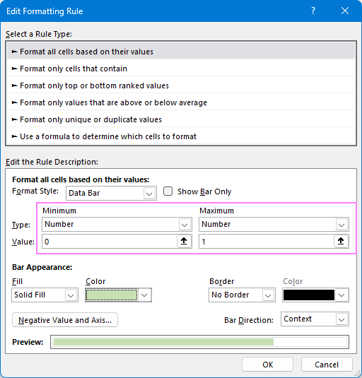
- Under Edit the Rule Description, you'll notice that, by default, Excel uses Automatic for the Minimum and Maximum values. For the bars to reflect the progress accurately, change both types to Number and enter 0 for Minimum and 1 for Maximum.
- To show only the bars without percentage values, select the Show Bar Only box.
- Choose a color that fits your spreadsheet design.
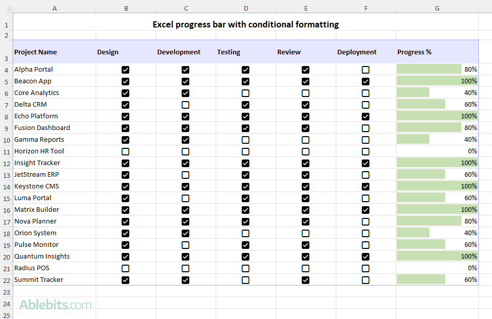
Now, you have a simple horizontal progress bar in each row that updates in real time as you check off milestones.
For more information, see How to add and customize Date Bars in Excel.
Create an overall progress bar for all tasks
The Data Bars method also works nicely for a vertical layout, where you have a list of tasks in one column and checkboxes in another column indicating whether a certain task is complete or not.
To display the overall progress for the entire list, you can calculate the percentage of completed tasks in a single cell at the top or bottom of your dataset.
For example, with checkboxes in B4:B14, we put this formula in B17:
=COUNTIF(B4:B14, TRUE) / COUNTA(B4:B14)
Next, apply Data Bars to that cell, just as described above. For the bar to display the progress correctly, make sure to set the value types to Number, with 0 and 1 as their Minimum and Maximum values. For details, see Step 5 in the previous section.
As a result, you'll get a neat, single-cell progress bar showing total completion for the whole list.
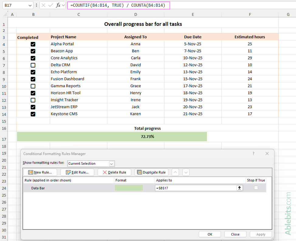
Tip. To make your progress bar bigger, you can merge a few adjacent cells in the same row as shown in the image above.
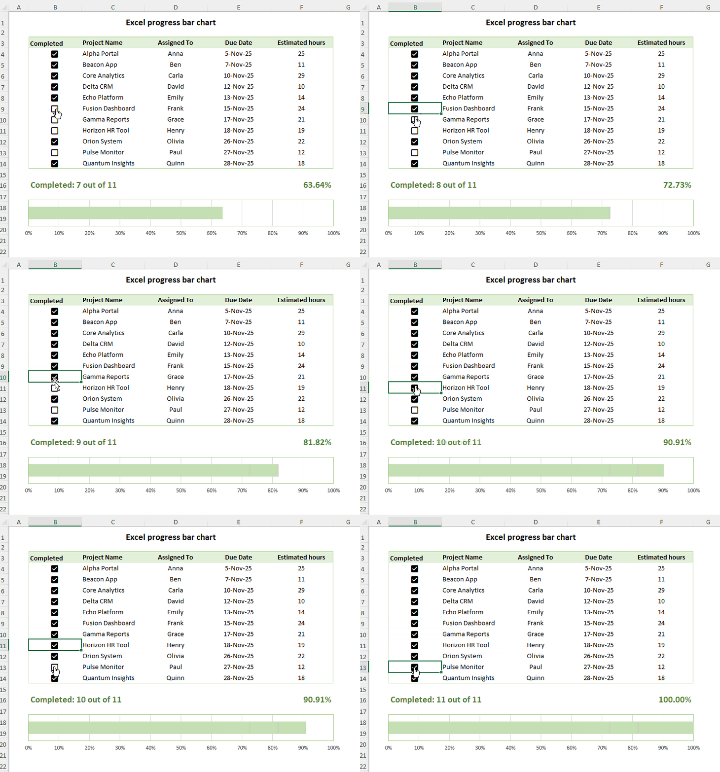
How to create progress bar chart in Excel
If you want to visualize completion in a professional format, a progress bar chart is an excellent choice. Just like the previous example, this one is also based on checkboxes.
Here's how to build it step-by-step:
- Insert checkboxes. For each item in your list, add a checkbox to indicate whether the task is complete.
- Link checkboxes to cells. If you use Check Box Form Controls, link each one to a separate cell. The new checkboxes in Excel 365 don't require any linking, as they automatically return TRUE or FALSE values in their own cells.
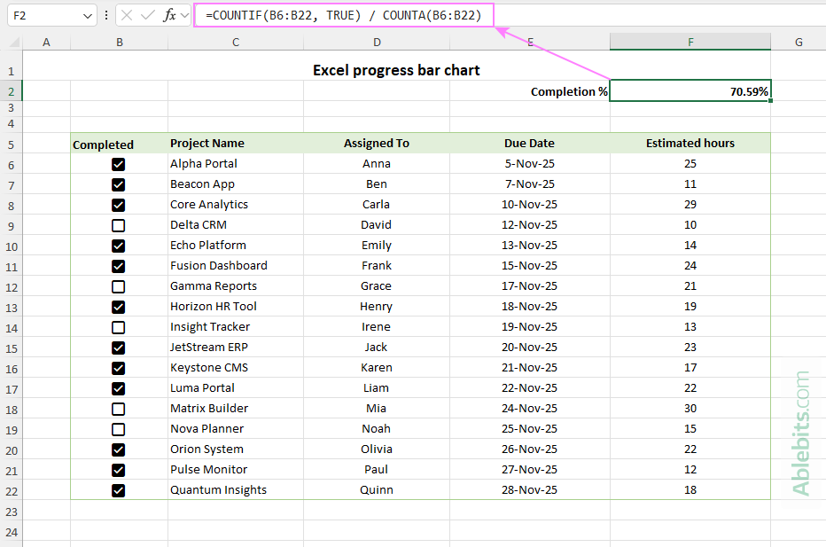
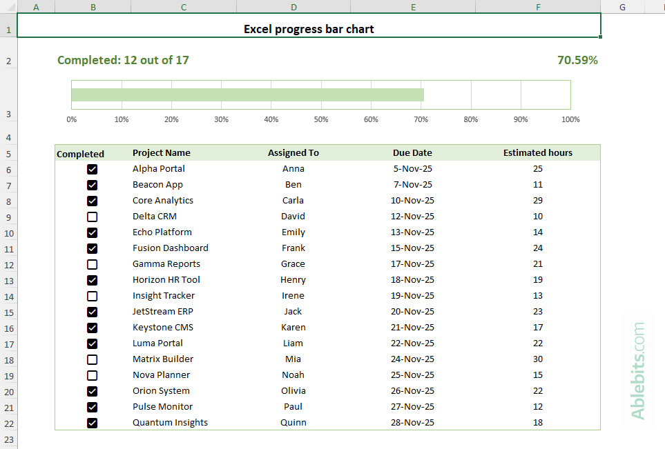
- Enter the completion percentage formula. Now, calculate the percentage of completed tasks. In any empty cell, enter the formula that counts the number of checked boxes. In this example, the following formula goes to cell F2:
=COUNTIF(B6:B22, TRUE) / COUNTA(B6:B22)
Where B6:B22 are cells with checkboxes.
- Insert a bar chart. Next, we'll turn that percentage into a visual progress bar.
- Select the cell with your percentage formula (F2 in our case).
- On the Insert tab, in the Charts group, click Insert Column or Bar Chart, and choose 2-D Bar.
Excel will insert a standard bar chart that represents your completion value. To properly reflect progress, the bar chart requires some essential customizations.
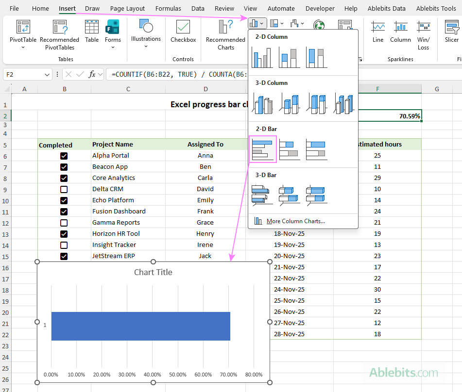
- Remove unnecessary chart elements. To make it look cleaner, remove extra elements such as the chart title and primary vertical axis. Optionally, you can also remove gridlines if you prefer a minimal look. For this, click the Chart Elements button in the upper-right corner of the graph, and tick or untick the desired boxes.

- Format the axis. To make sure your chart axis accurately reflects percentages, right-click the horizontal axis and choose Format Axis. In the Axis Options pane:
- Set Minimum bound to 0 and Maximum bound to 1, so the axis scale is from 0% to 100%.
- Adjust the Major and Minor units. For example, you can set Major Unit to 0.1 for 10% scale interval.
- Under Number, set Decimal places to 0 to show whole percentages.
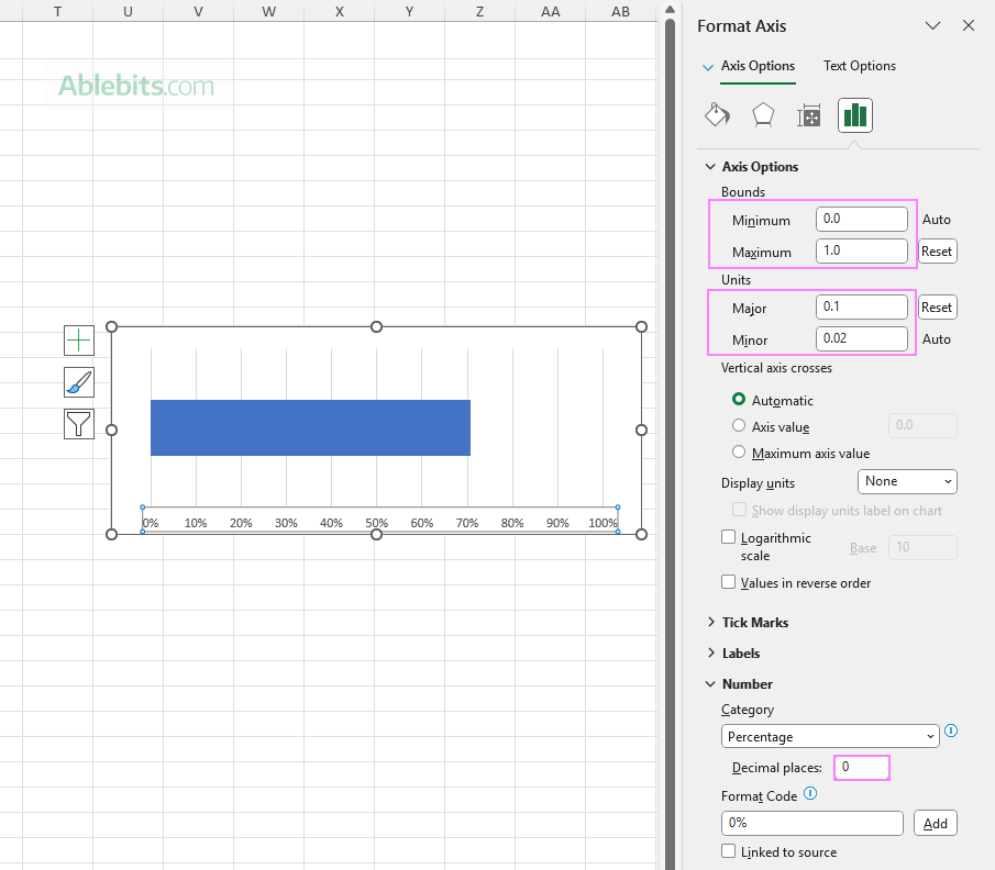
Basically, that's all you need to get your Excel progress bar chart working correctly. But if you want it to look as good as it functions, you can also make a few design improvements.
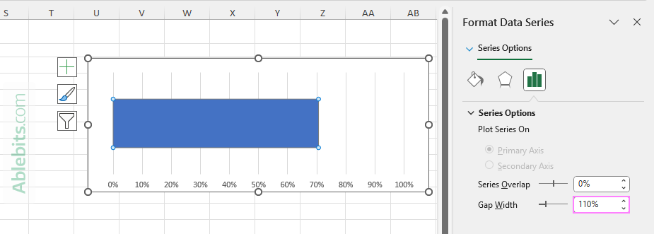
- Change the bar width. To make the progress bar thicker or narrower, right-click it in your graph and choose Format Data Series. In the Series Options pane, adjust the Gap Width slider or enter a value between 0% and 500% in the box. Lower values make the bar thicker, while higher values make it thinner.
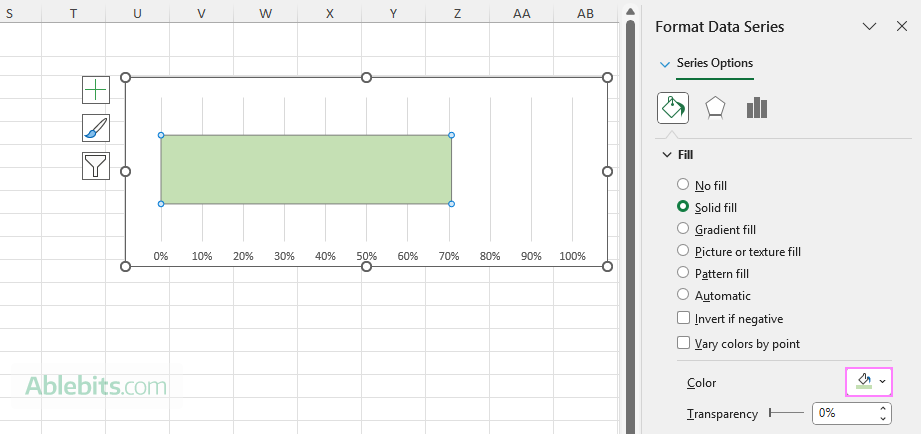
- Change the bar color. Set your preferred color for the bar. On the Format Data Series pane, switch to the Fill tab and choose a solid or gradient color you like.
- Apply final design improvements. Make any other customizations to refine your progress bar appearance. For example, you may want to:
- Remove the chart border: Right-click the chart area > Format Chart Area > under Border, choose No line.
- Add a border to the plot area: Right-click inside the plot area > Format Plot Area > under Border, select Solid line and pick a color that complements your progress bar.
- Adjust the chart size by dragging its vertical and horizontal borders.
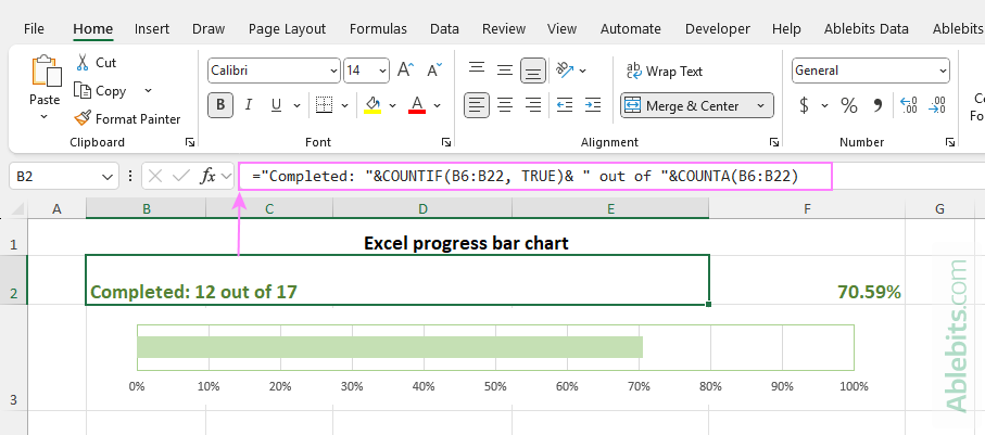
- Add a completion formula (optional). For a quick textual summary, you can add a formula showing how many tasks are done out of the total. To build it, we:
- Count the number of checked boxes: COUNTIF(B6:B22, TRUE)
- Count the total number of checkboxes: COUNTA(B6:B22)
- And concatenate both functions in a single formula:
="Completed: "&COUNTIF(B6:B22, TRUE)& " out of "&COUNTA(B6:B22)
You can place this formula just above or below your chart, and it will display a progress summary like shown in the screenshot below.
And that's it - your Excel progress bar chart is ready! It not only reflects task completion accurately but also adds a polished, dashboard-style touch to your progress tracker.
How to build circular charts for Excel progress trackers
If you prefer a circular progress display, you can easily create a doughnut or pie chart to show how much of your work is completed. The process is quite similar to building a progress bar chart. Here's a quick rundown to help you set it up.
Step 1. Write formulas for completed and uncompleted tasks
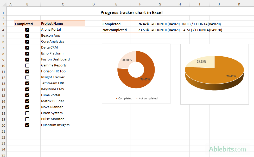
First, calculate how many tasks are done and how many remain. Assuming your checkboxes are in B4:B20, enter these formulas:
In F3, to count checked boxes:
=COUNTIF(B4:B20, TRUE)
In F4, to count unchecked boxes:
=COUNTIF(B4:B20, FALSE)
Alternatively, if you'd rather have percentage values, you can use:
Completed tasks:
=COUNTIF(B4:B20, TRUE) / COUNTA(B4:B20)
Pending tasks:
=COUNTIF(B4:B20, FALSE) / COUNTA(B4:B20)
Either approach will work. The choice depends on whether you want to display actual counts or percentages.
Step 2. Insert a doughnut or pie chart
Select both formula cells (F3 and F4 in this example). Then, go to the Insert tab and, in the Charts group, choose doughnut chart or pie graph if you prefer. Excel will instantly create a selected chart type showing completed vs. remaining tasks.
Step 3. Customize your chart
Unlike the progress bar chart, this one works well right out of the box, though a few formatting touches can make it look even better:
- Shade the completed portion in your main color and the uncompleted slice with a light neutral color. For detailed instructions, see how to change pie graph colors.
- Remove the chart title and legend for a minimalistic appearance.
- Optionally, add data labels showing the completion percentage.
That's all it takes! With a few quick tweaks, you've turned a simple checklist into a nice progress tracker chart that updates as you work.
You now know several ways to turn plain numbers and checkboxes into dynamic visual trackers. Use conditional formatting for simple in-cell data bars, create a progress bar chart for a more detailed look, or add a doughnut graph for a compact display. Ready to give it a try? Download our practice workbook below and experiment with each method yourself.
Practice workbook for download
Excel progress bar - examples (.xlsx file)
 by
by