The tutorial explains the basics of regression analysis and shows a few different ways to do linear regression in Excel.
Imagine this: you are provided with a whole lot of different data and are asked to predict next year's sales numbers for your company. You have discovered dozens, perhaps even hundreds, of factors that can possibly affect the numbers. But how do you know which ones are really important? Run regression analysis in Excel. It will give you an answer to this and many more questions: Which factors matter and which can be ignored? How closely are these factors related to each other? And how certain can you be about the predictions?
Regression analysis in Excel - the basics
In statistical modeling, regression analysis is used to estimate the relationships between two or more variables:
Dependent variable (aka criterion variable) is the main factor you are trying to understand and predict.
Independent variables (aka explanatory variables, or predictors) are the factors that might influence the dependent variable.
Regression analysis helps you understand how the dependent variable changes when one of the independent variables varies and allows to mathematically determine which of those variables really has an impact.
Technically, a regression analysis model is based on the sum of squares, which is a mathematical way to find the dispersion of data points. The goal of a model is to get the smallest possible sum of squares and draw a line that comes closest to the data.
In statistics, they differentiate between a simple and multiple linear regression. Simple linear regression models the relationship between a dependent variable and one independent variables using a linear function. If you use two or more explanatory variables to predict the dependent variable, you deal with multiple linear regression. If the dependent variable is modeled as a non-linear function because the data relationships do not follow a straight line, use nonlinear regression instead. The focus of this tutorial will be on a simple linear regression.
As an example, let's take sales numbers for umbrellas for the last 24 months and find out the average monthly rainfall for the same period. Plot this information on a chart, and the regression line will demonstrate the relationship between the independent variable (rainfall) and dependent variable (umbrella sales):
Mathematically, a linear regression is defined by this equation: Where: The linear regression equation always has an error term because, in real life, predictors are never perfectly precise. However, some programs, including Excel, do the error term calculation behind the scenes. So, in Excel, you do linear regression using the least squares method and seek coefficients a and b such that: For our example, the linear regression equation takes the following shape: There exist a handful of different ways to find a and b. The three main methods to perform linear regression analysis in Excel are: Below you will find the detailed instructions on using each method.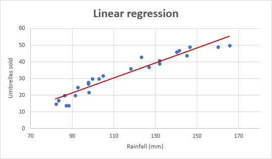
Linear regression equation
Umbrellas sold = b * rainfall + a
How to do linear regression in Excel with Analysis ToolPak
This example shows how to run regression in Excel by using a special tool included with the Analysis ToolPak add-in.
Enable the Analysis ToolPak add-in
Analysis ToolPak is available in all versions of Excel 365 to 2003 but is not enabled by default. So, you need to turn it on manually. Here's how:
- In your Excel, click File > Options.
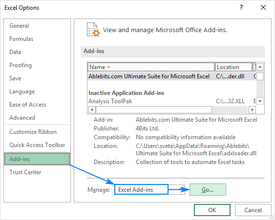
- In the Excel Options dialog box, select Add-ins on the left sidebar, make sure Excel Add-ins is selected in the Manage box, and click Go.
- In the Add-ins dialog box, tick off Analysis Toolpak, and click OK:

This will add the Data Analysis tools to the Data tab of your Excel ribbon.
Run regression analysis
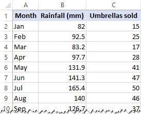
In this example, we are going to do a simple linear regression in Excel. What we have is a list of average monthly rainfall for the last 24 months in column B, which is our independent variable (predictor), and the number of umbrellas sold in column C, which is the dependent variable. Of course, there are many other factors that can affect sales, but for now we focus only on these two variables:
With Analysis Toolpak added enabled, carry out these steps to perform regression analysis in Excel:
- On the Data tab, in the Analysis group, click the Data Analysis button.

- Select Regression and click OK.

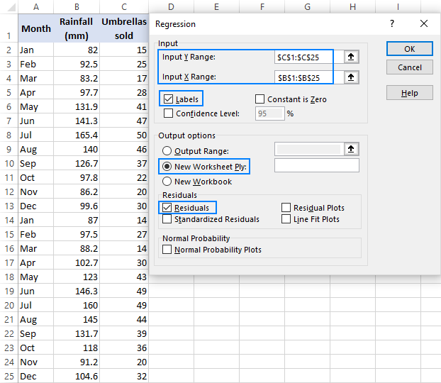
- In the Regression dialog box, configure the following settings:
- Select the Input Y Range, which is your dependent variable. In our case, it's umbrella sales (C1:C25).
- Select the Input X Range, i.e. your independent variable. In this example, it's the average monthly rainfall (B1:B25).
If you are building a multiple regression model, select two or more adjacent columns with different independent variables.
- Check the Labels box if there are headers at the top of your X and Y ranges.
- Choose your preferred Output option, a new worksheet in our case.
- Optionally, select the Residuals checkbox to get the difference between the predicted and actual values.
- Click OK and observe the regression analysis output created by Excel.
Interpret regression analysis output
As you have just seen, running regression in Excel is easy because all calculations are preformed automatically. The interpretation of the results is a bit trickier because you need to know what is behind each number. Below you will find a breakdown of 4 major parts of the regression analysis output.
Regression analysis output: Summary Output
This part tells you how well the calculated linear regression equation fits your source data.

Here's what each piece of information means:
Multiple R. It is the Correlation Coefficient that measures the strength of a linear relationship between two variables. The correlation coefficient can be any value between -1 and 1, and its absolute value indicates the relationship strength. The larger the absolute value, the stronger the relationship:
- 1 means a strong positive relationship
- -1 means a strong negative relationship
- 0 means no relationship at all
R Square. It is the Coefficient of Determination, which is used as an indicator of the goodness of fit. It shows how many points fall on the regression line. The R2 value is calculated from the total sum of squares, more precisely, it is the sum of the squared deviations of the original data from the mean.
In our example, R2 is 0.91 (rounded to 2 digits), which is fairy good. It means that 91% of our values fit the regression analysis model. In other words, 91% of the dependent variables (y-values) are explained by the independent variables (x-values). Generally, R Squared of 95% or more is considered a good fit.
Adjusted R Square. It is the R square adjusted for the number of independent variable in the model. You will want to use this value instead of R square for multiple regression analysis.
Standard Error. It is another goodness-of-fit measure that shows the precision of your regression analysis - the smaller the number, the more certain you can be about your regression equation. While R2 represents the percentage of the dependent variables variance that is explained by the model, Standard Error is an absolute measure that shows the average distance that the data points fall from the regression line.
Observations. It is simply the number of observations in your model.
Regression analysis output: ANOVA
The second part of the output is Analysis of Variance (ANOVA):

Basically, it splits the sum of squares into individual components that give information about the levels of variability within your regression model:
- df is the number of the degrees of freedom associated with the sources of variance.
- SS is the sum of squares. The smaller the Residual SS compared with the Total SS, the better your model fits the data.
- MS is the mean square.
- F is the F statistic, or F-test for the null hypothesis. It is used to test the overall significance of the model.
- Significance F is the P-value of F.
The ANOVA part is rarely used for a simple linear regression analysis in Excel, but you should definitely have a close look at the last component. The Significance F value gives an idea of how reliable (statistically significant) your results are. If Significance F is less than 0.05 (5%), your model is OK. If it is greater than 0.05, you'd probably better choose another independent variable.
Regression analysis output: coefficients
This section provides specific information about the components of your analysis:

The most useful component in this section is Coefficients. It enables you to build a linear regression equation in Excel:
For our data set, where y is the number of umbrellas sold and x is an average monthly rainfall, our linear regression formula goes as follows:
Y = Rainfall Coefficient * x + Intercept
Equipped with a and b values rounded to three decimal places, it turns into:
Y=0.45*x-19.074
For example, with the average monthly rainfall equal to 82 mm, the umbrella sales would be approximately 17.8:
0.45*82-19.074=17.8
In a similar manner, you can find out how many umbrellas are going to be sold with any other monthly rainfall (x variable) you specify.
Regression analysis output: residuals
If you compare the estimated and actual number of sold umbrellas corresponding to the monthly rainfall of 82 mm, you will see that these numbers are slightly different:
- Estimated: 17.8 (calculated above)
- Actual: 15 (row 2 of the source data)
Why's the difference? Because independent variables are never perfect predictors of the dependent variables. And the residuals can help you understand how far away the actual values are from the predicted values:

For the first data point (rainfall of 82 mm), the residual is approximately -2.8. So, we add this number to the predicted value, and get the actual value: 17.8 - 2.8 = 15.
How to make a linear regression graph in Excel
If you need to quickly visualize the relationship between the two variables, draw a linear regression chart. That's very easy! Here's how:
- Select the two columns with your data, including headers.
- On the Inset tab, in the Chats group, click the Scatter chart icon, and select the Scatter thumbnail (the first one):
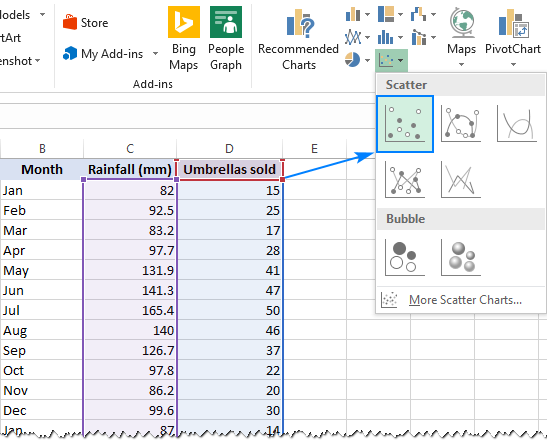
This will insert a scatter plot in your worksheet, which will resemble this one:

- Now, we need to draw the least squares regression line. To have it done, right click on any point and choose Add Trendline… from the context menu.

- On the right pane, select the Linear trendline shape and, optionally, check Display Equation on Chart to get your regression formula:
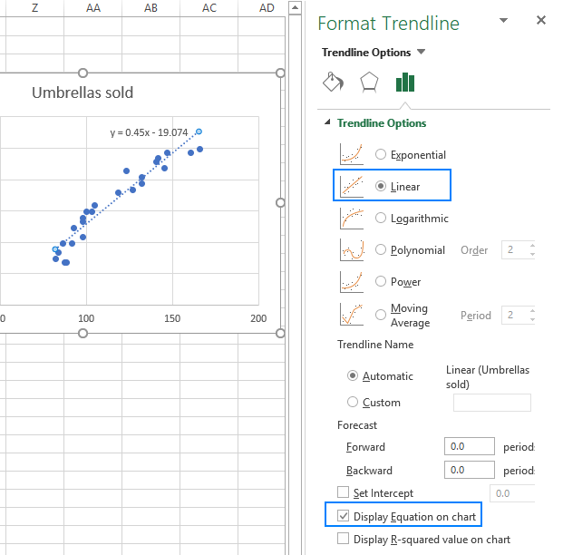
As you may notice, the regression equation Excel has created for us is the same as the linear regression formula we built based on the Coefficients output.
- Switch to the Fill & Line tab and customize the line to your liking. For example, you can choose a different line color and use a solid line instead of a dashed line (select Solid line in the Dash type box):

At this point, your chart already looks like a decent regression graph:

Still, you may want to make a few more improvements:
- Drag the equation wherever you see fit.
- Add axes titles (Chart Elements button > Axis Titles).
- If your data points start in the middle of the horizontal and/or vertical axis like in this example, you may want to get rid of the excessive white space. The following tip explains how to do this: Scale the chart axes to reduce white space.
And this is how our improved regression graph looks like:
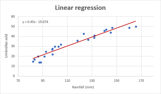
Important note! In the regression graph, the independent variable should always be on the X axis and the dependent variable on the Y axis. If your graph is plotted in the reverse order, swap the columns in your worksheet, and then draw the chart anew. If you are not allowed to rearrange the source data, then you can switch the X and Y axes directly in a chart.
How to do regression in Excel using formulas
Microsoft Excel has a few statistical functions that can help you to do linear regression analysis such as LINEST, SLOPE, INTERCEPT, and CORREL.
The LINEST function uses the least squares regression method to calculate a straight line that best explains the relationship between your variables and returns an array describing that line. You can find the detailed explanation of the function's syntax in this tutorial. For now, let's just make a formula for our sample dataset:
=LINEST(C2:C25, B2:B25)
Because the LINEST function returns an array of values, you must enter it as an array formula. Select two adjacent cells in the same row, E2:F2 in our case, type the formula, and press Ctrl + Shift + Enter to complete it.
The formula returns the b coefficient (E1) and the a constant (F1) for the already familiar linear regression equation:
y = bx + a

If you avoid using array formulas in your worksheets, you can calculate a and b individually with regular formulas:
Get the Y-intercept (a):
=INTERCEPT(C2:C25, B2:B25)
Get the slope (b):
=SLOPE(C2:C25, B2:B25)
Additionally, you can find the correlation coefficient (Multiple R in the regression analysis summary output) that indicates how strongly the two variables are related to each other:
=CORREL(B2:B25,C2:C25)
The following screenshot shows all these Excel regression formulas in action:

Tip. If you'd like to get additional statistics for your regression analysis, use the LINEST function with the stats parameter set to TRUE as shown in this example.
That's how you do linear regression in Excel. That said, please keep in mind that Microsoft Excel is not a statistical program. If you need to perform regression analysis at the professional level, you may want to use targeted software such as XLSTAT, RegressIt, etc.
To have a closer look at our linear regression formulas and other techniques discussed in this tutorial, you are welcome to download our sample workbook below. Thank you for reading!
Practice workbook
Regression Analysis in Excel - examples (.xlsx file)
 by
by
152 comments
Helpful
Very good explanation with the excel formulae.
Hi, why does the R Square value derived by the RSQ function different from what is derived through the the Data Analysis function?
This was very useful and instructive , the example are very explicit and relatable to my current problem . Thanks for the help and i hope you continue your work. Well done
Foud this tutorial so helpful. Need to know how to do multiple regression. Thanks
Very helpful article
This write up was of great help to me. Thank you.
Why does the regression equation change from a + to a - of the intercept?
Well done for this article and thank you for mentioning that XLSTAT is a professional solution for doing linear regression.
A big thank you from the XLSTAT team! Nicolas
Very good blog,thank so much for your effort in writing the posts.
To whoever that has published this,
You just saved my life! I can't thank you enough! You'll prosper!!!
Good Job. Thank you very much.
Hmm, you are indeed a great teacher! How can I get this tutorial in PDF?
Thank you very much. I wish you more wins in all your affairs. Regards from Nigeria. ?
You are an absolute beast! Thank you so much. This helped a ton. Excel is so powerful!
very helpful
Thank you!! Svetlana Cheusheva
Mrs. Svetlana,
Thank you for this post, it really helped me. Now if you do not mind I would like to ask a further question. If the alpha value of this equation was 0.05, should I accept or reject the null hypothesis? Any help or guidance in this matter would be much appreciated. Thank you for your time.
Best Regards,
Justin
Super helpful! Thanks!
Thanks for sharing the ARTICLE. Very helpful
Thnak you for sharing this knowledge with us.
How can you calculate the average monthly rainfall in here ..
Hi Praful,
By using the AVERAGE function. And we have a detailed tutorial on this: How to calculate average (mean) in Excel
Very user friendly resource to understand.
Simple and easy to understand. Well explained. Thank you!
very interesting and precise guide.
Great job on equation types To .be used in régressions.
However in computing coefficient values, I cannot find the numeric equivalence of ^(1,2) in the formula, say,
LINEST(C2:C13,B2:B13^(1,2),1).
In other words, replacing the above two vactors by their row correspondance how does the above formula computes the coefficient values.
Thank you
Hi
How can I run the Data Analysis regression and ignore data inputs such as "-" in the middle of the data table?
This is the best clarification I have ever received in recent times. Thank you very much as this has just assisted with my data analysis for my MSc dissertation. I was at a crossroads until I saw this.
Thanks very much you are a saving grace.
thanks very much, it was very very helpful. it aided me complete my assignment.
thank you so much very helpful!
Thanks Ms, great introduction specially for excel regression model
well presented ,made so simple to get complete idea!
1.True or false: In simple regression analysis, if the intercept is negative, then there is a negative
correlation between the dependent variable and the independent variable .
2. True or false: The range of values that indicates that there is a significant difference between the
value of the sample statistic and the proposed parameter value is called the rejection
region.
Very nice explanation. I have data in row wise instead of column wise. I am unable to run the regression. Please can you help me out in performing regression with row wise data
Hello,
I would like to know the mathematical formulas that Excel uses to calculate the linear regression coefficients. Can you help me?
Umar
Thank you so much for this very clear and helpful tutorial! It was really excellent.
This was an amazing explanation, thank you very much ! :)
required to chart a linear regression line, but it makes creating statistics tables simpler. To verify if installed, select Data from the toolbar. If Data Analysis is an option, the feature is installed and ready to use. If not installed, you can request this option by clicking on the Office button and selecting Excel options .
I just want to say thank you for this well descriptive explanation of how to add in the data analysis, as well as explaining what to type in for the x and y ranges and what I could learn from the analysis once it was completed. This has helped me tremendously. Thank you!!!!
Thanks a lot....best explanation ever.
Thank you very much. The best explanation I've found. Wonderful!!!
Hi Svetlana. I never place my comments but your tutorial is worth it! All other pages either just show how its done or explain it very "statistically". But you explained it like teaching to a child. Thank you again for this!
Best explanation of regression ever. Very simple, clear and easy to understand. Thank you so much and will keep a tab on your tutorials.
thanks a lot. really helped.
Very well explained! Thanks.
Hi!
Also for me it was really helpful!
Unfortunately I cannot produce a graph for a multiple linear regression. Is Excel not able to show it or do you have a tutorial about it, which could help me?
Thanks!
This write-up has really helped me, but I'm left with one other question:
If I am using linear regression on a standard curve (say response over concentration) to obtain an equation that I can use to determine the concentration of unknown samples, how do I determine the uncertainty of the concentration value that this equation yields?
Thank you for this tutorial, it was a lifesaver!
I agree with Andre above. this is the clearest tutorial ever. So easy to follow.
Further question, how do you deal with blank spaces in the data? If I chart it, I can still get a trend line and equation but if I try to work directly from the data it balks.
Thank you very much
Wow, first excel tutorial I read that is clear from A to Z...nice!
Hi Svetlana,
I really like your explanations for linear regression, but I am confused about your explanation on Significance F value. In the example you provided, you explained that If Significance F is less than 0.05 (5%), your model is OK. If it is greater than 0.05, you'd probably better choose another independent variable.
But When responding to Ali's question whose Significance F value is 6.07596E-31, you said " in your case, Significance F is far less than 5%, so your results are statistically significant." So between (0.05) and (6.07), which one is greater than the other one?
I have run my regression and my Significance F value is 0.005590647. Is this value (0.005) greater or less than (0.05)?
Please, I am confused.
Hi!
6.07 is of course greater than 0.05. However, 6.07596E-31 is not 6.07, it is 0.000000000000000000000000000000607596! 6.07596E-31 is a special format (Scientific notation) used by Excel to display very large and very small numbers in a compact way. When responding to Ali's question I briefly explained about the Scientific format, you can find more info here: Scientific notation format in Excel.
In your case, Significance F (0.005590647) is also less than 0.05 - the more zeros after the decimal point the smaller the number.
Simple and well explained!