In this tutorial, you will learn 3 different ways to dynamically highlight the row and column of a selected cell in Excel.
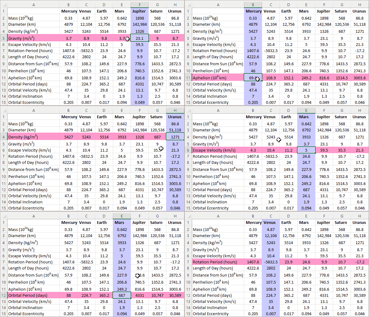
When viewing a large worksheet for a long time, you may eventually lose track of where your cursor is and which data you are looking at. To know exactly where you are at any moment, get Excel to automatically highlight the active row and column for you! Naturally, the highlighting should be dynamic and change every time you select another cell. Essentially, this is what we are aiming to achieve:
Auto-highlight row and column of selected cell with VBA
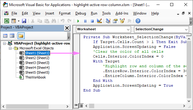
This example shows how you can highlight an active column and row programmatically with VBA. For this, we will be using the SelectionChange event of the Worksheet object.
First, you clear the background color of all cells on the sheet by setting the ColorIndex property to 0. And then, you highlight the entire row and column of the active cell by setting their ColorIndex property to the index number for the desired color.
Customizing the code
If you'd like to customize the code for your needs, these small tips may come in handy:
- Our sample code uses two different colors demonstrated in the above gif - color index 38 for row and 24 for column. To change the highlight color, just replace those with any ColorIndex codes of your choosing.
- To get the row and column colored in the same way, use the same color index number for both.
- To only highlight the active row, remove or comment out this line: .EntireColumn.Interior.ColorIndex = 24
- To only highlight the active column, remove or comment out this line: .EntireRow.Interior.ColorIndex = 38
How to add the code to your worksheet
To have the code silently executed in the background of a specific worksheet, you need to insert it in the code window belonging to that worksheet, not in the normal module. To have it done, carry out these steps:
- In your workbook, press Alt + F11 to get to the VBA editor.
- In the Project Explorer on the left, you'll see a list of all open workbooks and their worksheets. If you don't see it, use the Ctrl + R shortcut to bring the Project Explorer window to view.
- Find the target workbook. In its Microsoft Excel Objects folder, double-click on the sheet in which you want to apply highlighting. In this example, it's Sheet 1.
- In the Code window on the right, paste the above code.
- Save your file as Macro-Enabled Workbook (.xlsm).
Advantages: everything is done in the backend; no adjustments/customizations are needed on the user's side; works in all Excel versions.
Drawbacks: there are two essential downsides that make this technique inapplicable under certain circumstances:
- The code clears background colors of all cells in the worksheet. If you have any colored cells, do not use this solution because your custom formatting will be lost.
- Executing this code blocks the undo functionality on the sheet, and you won't be able to undo an erroneous action by pressing Ctrl + Z.
Highlight active row and column without VBA
The best you can get to highlight the selected row and/or column without VBA is Excel's conditional formatting. To set it up, carry out these steps:
- Select your dataset in which the highlighting should be done.
- On the Home tab, in the Styles group, click New Rule.
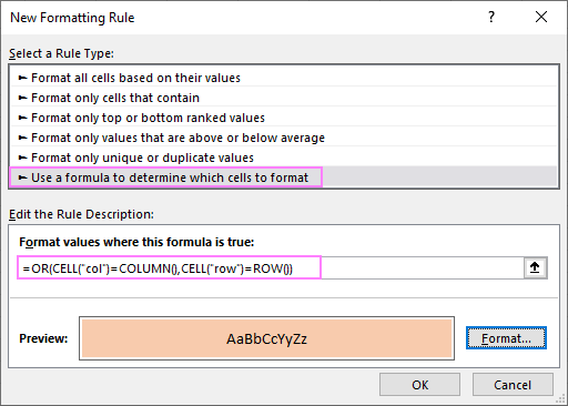
- In the New Formatting Rule dialog box, choose Use a formula to determine which cells to format.
- In the Format values where this formula is true box, enter one of these formulas:
To highlight active row:
=CELL("row")=ROW()To highlight active column:
=CELL("col")=COLUMN()To highlight active row and column:
=OR(CELL("row")=ROW(), CELL("col")= COLUMN())All the formulas make use of the CELL function to return the row/column number of the selected cell.
- Click the Format button, switch to the Fill tab, and select the color you like.
- Click OK twice to close both dialog windows.
If you feel like you need more detailed instructions, please see How to create formula-based conditional formatting rule.
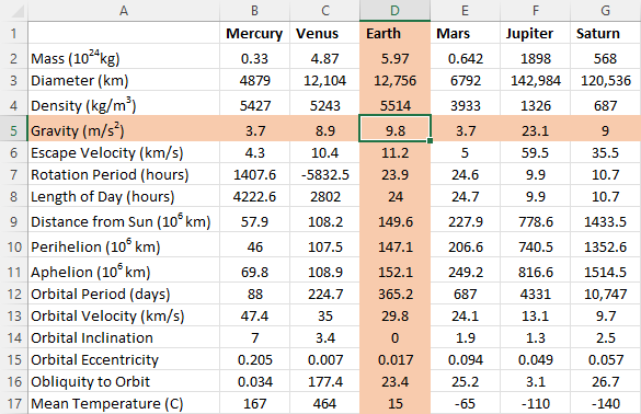
For this example, we opted for the OR formula to shade both the column and row in the same color. That takes less work and is suitable for most cases.
Unfortunately, this solution is not as nice as the VBA one because it requires recalculating the sheet manually (by pressing the F9 key). By default, Excel recalculates a worksheet only after entering new data or editing the existing one, but not when the selection changes. So, you select another cell - nothing happens. Press F9 - the sheet is refreshed, the formula is recalculated, and the highlighting is updated.
To get the worksheet recalculated automatically whenever the SelectionChange event occurs, you can place this simple VBA code in the code module of your target sheet as explained in the previous example:
The code forces the selected range/cell to recalculate, which in turn forces the CELL function to update and the conditional formatting to reflect the change.
Advantages: unlike the previous method, this one does not impact the existing formatting you have applied manually.
Drawbacks: may worsen Excel's performance.
- For the conditional formatting to work, you need to force Excel to recalculate the formula on every selection change (either manually with the F9 key or automatically with VBA). Forced recalculations may slow down your Excel. Since our code recalculates the selection rather than an entire sheet, a negative effect will most likely be noticeable only on really large and complex workbooks.
- Since the CELL function is available in Excel 2007 and higher, the method won't work in earlier versions.
Highlight selected row and column using conditional formatting and VBA
In case the previous method slows down your workbook considerably, you can approach the task differently - instead of recalculating a worksheet on every user move, get the active row/column number with the help of VBA, and then serve that number to the ROW() or COLUMN() function by using conditional formatting formulas.
To accomplish this, here are the steps you need to follow:
- Add a new blank sheet to your workbook and name it Helper Sheet. The only purpose of this sheet is to store two numbers representing the row and column containing a selected cell, so you can safely hide the sheet at a later point.
- Insert the below VBA in the code window of the worksheet where you wish to implement highlighting. For the detailed instructions, please refer to our first example.
Private Sub Worksheet_SelectionChange(ByVal Target As Range) Application.ScreenUpdating = False Worksheets("Helper Sheet").Cells(2, 1) = Target.Row Worksheets("Helper Sheet").Cells(2, 2) = Target.Column Application.ScreenUpdating = True End Sub
The above code places the coordinates of the active row and column to the sheet named "Helper Sheet". If you named your sheet differently in step 1, change the worksheet name in the code accordingly. The row number is written to A2 and the column number to B2.
- In your target worksheet, select the entire dataset, and create a conditional formatting rule with the below formulas. The step-by-step guidance is provided in the above example.
And now, let's cover the three main use cases in detail.
How to highlight active row
To highlight the row where your cursor is placed at the moment, set up a conditional formatting rule with this formula:
=ROW()='Helper Sheet'!$A$2

As the result, the user can clearly see which row is currently selected:

How to highlight active column
To highlight the selected column, feed the column number to the COLUMN function using this formula:
=COLUMN()='Helper Sheet'!$B$2
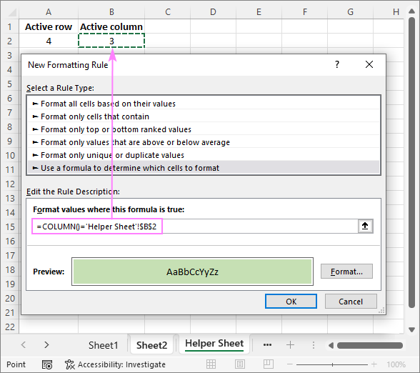
Now, a highlighted column lets you comfortably and effortlessly read vertical data focusing entirely on it.

How to highlight active row and column
To get both the selected row and column automatically shaded in the same color, combine the ROW() and COLUMN() functions into one formula:
=OR(ROW()='Helper Sheet'!$A$2, COLUMN()='Helper Sheet'!$B$2)
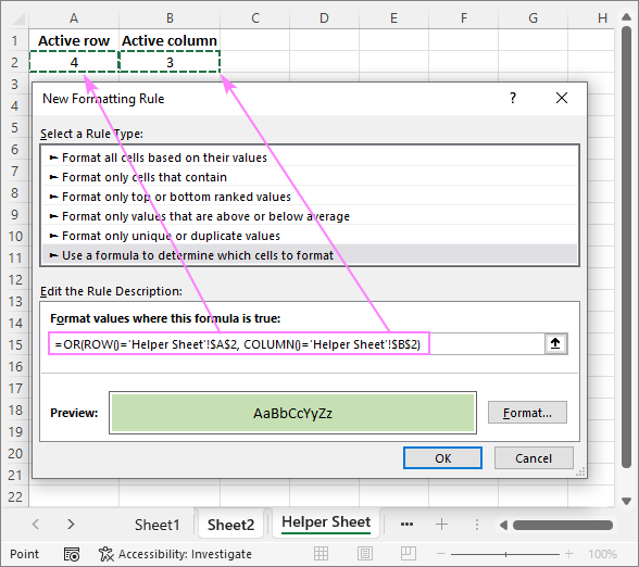
The relevant data is immediately brought into focus, so you can avoid misreading it.
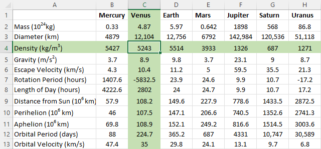
Advantages: optimized performance; works in all Excel versions
Drawbacks: the longest setup
Focus cell in Excel 365
In Excel 365 and Excel 2024 (version 2410 or later for Windows), there's no need for VBA and complex workarounds to track your current position on the sheet – the Focus Cell feature handles it for you automatically.
The Focus Cell highlights both the row and column of the active cell, giving you a clear visual cue of where you're working. Here's how to enable it:
- In Excel 365, go to the View tab.
- In the Show group, click the Focus Cell button.
That's it! The highlighting appears instantly around the active cell's row and column.
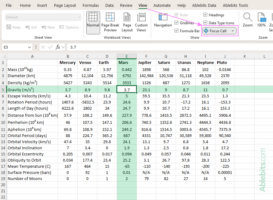
Prefer using the keyboard? You can turn on Focus Cell with these sequential key presses: Alt + W + E + F
- Alt - displays the ribbon key tips / shortcuts.
- W - opens the View tab.
- E – opens the Focus Cell menu.
- F – turns on the Focus Cell feature.
By default, Excel uses green for the highlight, but you can change it to a color that suits your preference:
- On the View tab, click the dropdown arrow next to the Focus Cell button.
- Select Focus Cell Color from the dropdown.
- Pick your desired color from the palette.
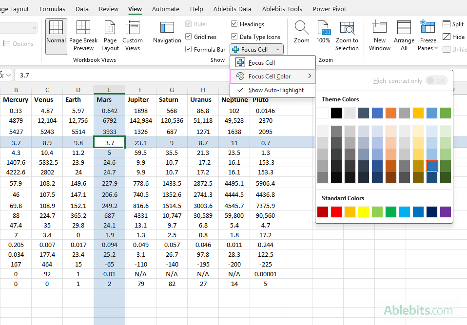
Excel remembers your selection. The next time you turn the feature back on, your custom color will still be in use.
Tip. When you use Find or Replace, Excel automatically turns on Focus Cell so you can easily spot the current cell as it shifts the position. If you'd rather turn off this auto-highlight, go to View > Focus Cell and uncheck Show Auto-Highlight.
Advantages: quick, built-in, and doesn't need extra setup
Limitations: is not available in older Excel versions ; can't set different colors for the row and column highlights
That's how to highlight the column and row of a selected cell in Excel. I thank you for reading and look forward to seeing you on our blog next week!
Practice workbook for download
Highlighting active row and column (.xlsm file)
 by
by
13 comments
My Excel has color on most pages, is there a way to highlight without removing all existing highlighted/colored cells?
Hi Bella,
If you are using Excel 365 or 2024, then you can leverage the built-in Focus Cell feature, which is a simple one-click action. In older versions, you can try the method described in the "Highlight active row and column without VBA" section, which does not affect existing colored cells.
Hello,
I used to have this tool in some documents using the conditional formatting solution. Suddenly it doesn't work. I actually have to press manually on F9 to see the change. What could have changed whereas I didn't change anything ? (or at least purposely)
It looks like the Excel settings have changed on their own.
Thanks for your feedback.
JJ
Hi! Changing the cell color and cell format does not cause Excel to automatically recalculate formulas, because the values in the cells are not changed.
In addition, I can't see your Excel settings.
its is included in excel now, called focus cell!
It’s vanishing other cell color as well. Is there any way to highlight column/row without hampering other cell color?
Hi! Conditional formatting changes the color of all cells in a row or column. Specify the range of the conditional formatting, not the entire column or row, if you do not want to change the color of some cells.
Tahnks so much, I think there is an error in one of the images, just below the text
How to highlight active row
To highlight the row where your cursor is placed at the moment, set up a conditional formatting rule with this formula:
=ROW()='Helper Sheet'!$A$2
The image shows different code - i.e. = CELL("row").... I think it should show as above =ROW().... thanks again. Just thought I'd share as it threw me for a bit.
Hi Anthony,
You are right - the formula in the screenshot was indeed incorrect (somehow got there from the previous example). Fixed, thank you very much for pointing to this!
hi! love this thank you for sharing. I like setting up macros for formulas etc.. that I use often and this would be one that I would like to have as a permanent macro in my "personal" file so that I can activate the macro to any sheet I use. do you have any suggestions on how to get that done?
thanks!!
Hi! Here is the article that may be helpful to you: Personal Macro Workbook in Excel - make macros available in all workbooks.
Hi. I was wondering if this highlight function (for the active row and column of the selected cell) is readily available in your Excel add-on?
Thanks.
Hello!
Our Ultimate Suite for Excel does not include this feature. But there are 70+ professional tools with 300+ options, among which you can find useful ones for yourself. You can read more details on this page.