Whether there's summer knocking on our doors or winter invading Westeros, we still work in Google Sheets and have to compare different pieces of tables with one another. In this article, I'm sharing ways of matching your data and giving away tips on doing that swiftly.
Compare two columns or sheets
One of the tasks you may have is to scan two columns or sheets for matches or differences and identify them somewhere outside the tables.
Compare two columns in Google Sheets for matches and differences
I'll start by comparing two cells in Google Sheets. This way lets you scan entire columns row by row.
Example 1. Google Sheets – compare two cells
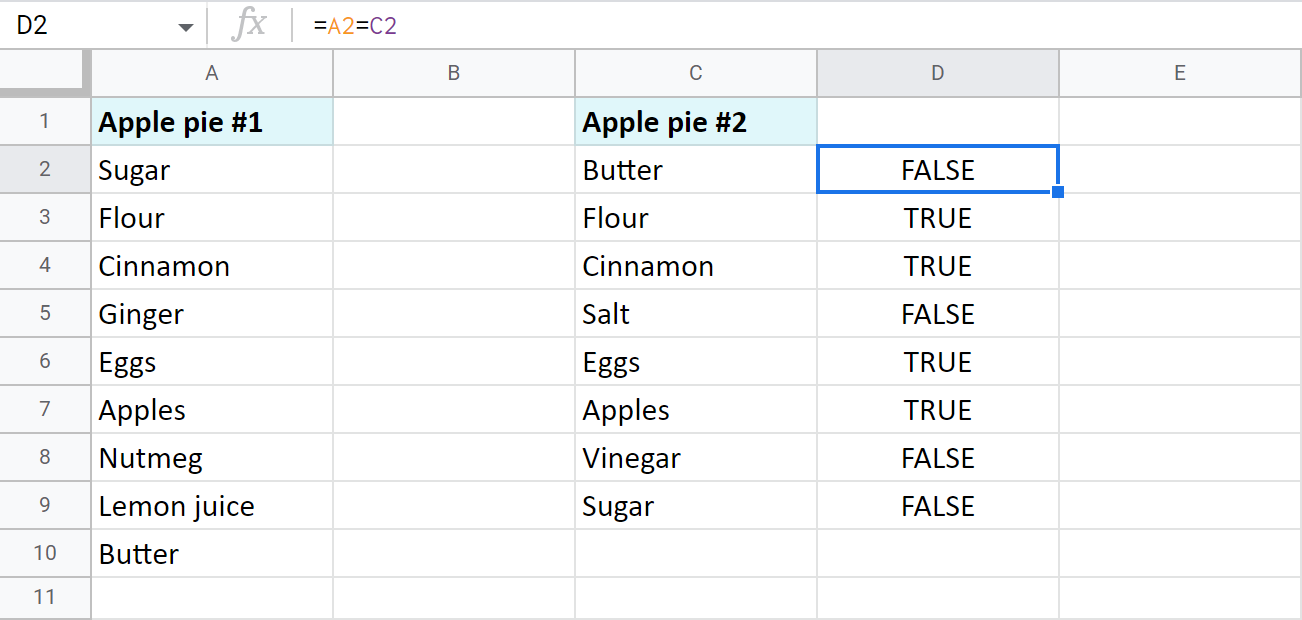
For this first example, you will need a helper column in order to enter the formula into the first row of the data to compare:
=A2=C2
If cells match, you'll see TRUE, otherwise FALSE. To check all cells in a column, copy the formula down to other rows:
Tip. To compare columns from different files, you need to use the IMPORTRANGE function:
=A2=IMPORTRANGE("spreadsheet_url","Sheet1!A2")
Example 2. Google Sheets – compare two lists for matches and differences
- A neater solution would be to use the IF function. You'll be able to set the exact status for identical and different cells:
=IF(A2=C2,"Match","Differ")
Tip. If your data is written in different cases and you'd like to consider such words as different, here's the formula for you:
=IF(EXACT(A2,C2),"Match","Differ")Where EXACT considers the case and looks for the complete identicals.
- To identify only rows with duplicate cells, use this formula:
=IF(A2=C2,"Match","") - To mark only rows with unique records between cells in two columns, take this one:
=IF(A2=C2,"","Differ")
Example 3. Compare two columns in Google Sheets
-
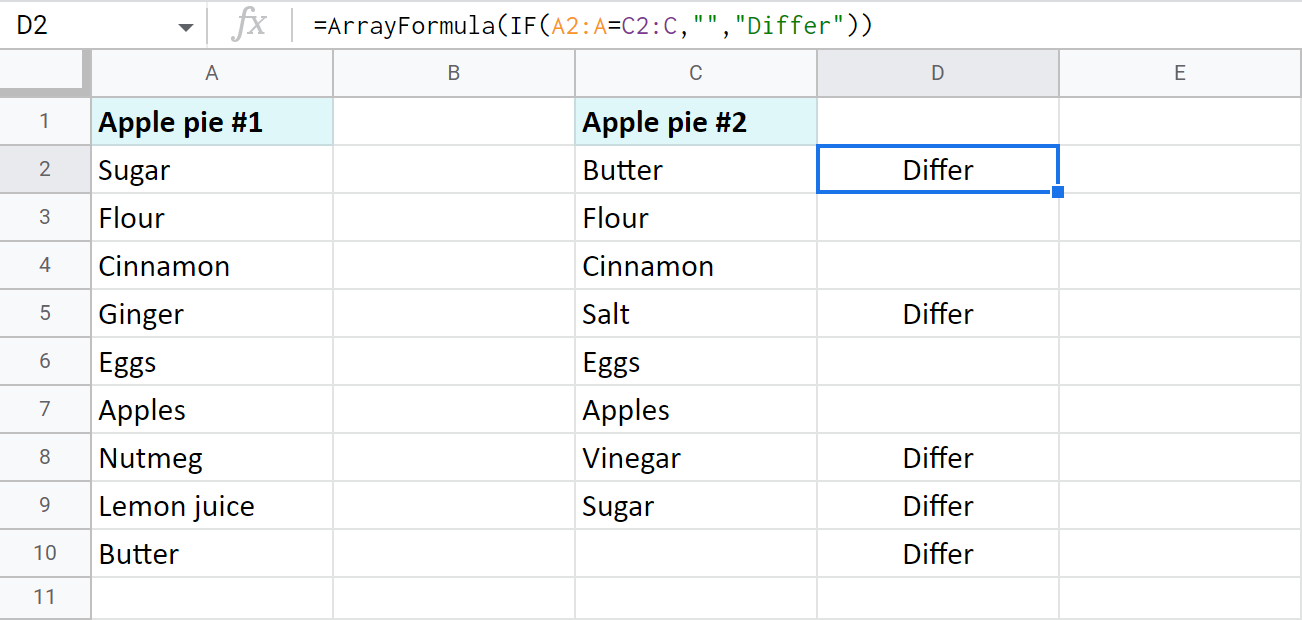
There's a way to avoid copying the formula over each row. You can forge an array IF formula in the first cell of your helper column:
=ArrayFormula(IF(A2:A=C2:C,"","Differ"))This IF pairs each cell of column A with the same row in column C. If records are different, the row will be identified accordingly. What is nice about this array formula is that it automatically marks each and every row at once:
-
In case you'd rather name the rows with identical cells, fill the second argument of the formula instead of the third one:
=ArrayFormula(IF(A2:A=C2:C,"Match",""))
Example 4. Compare two Google Sheets for differences
Oftentimes you need to compare two columns in Google Sheets that belong inside a huge table. Or they can be entirely different sheets like reports, price lists, working shifts per month, etc. Then, I believe, you can't afford to create a helper column or it can be quite difficult to manage.
If this sounds familiar, don't worry, you can still mark the differences on another sheet.
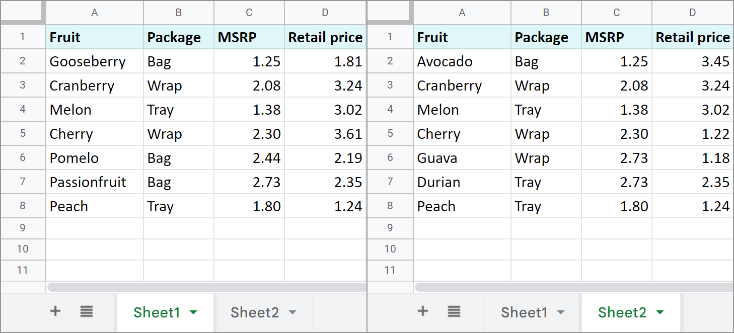
Here are two tables with products and their prices. I want to locate all cells with different contents between these tables:
Start with creating a new sheet and enter the next formula into A1:
=IF(Sheet1!A1<>Sheet2!A1,Sheet1!A1&" | "&Sheet2!A1,"")
Note. You must copy the formula over the range equal to the size of the biggest table.
As a result, you will see only those cells that differ in contents. The formula will also pull records from both tables and separate them with a character you enter into the formula:

Tip. If the sheets to compare are in different files, again, just incorporate the IMPORTRANGE function:
=IF(Sheet1!A1<>IMPORTRANGE("2nd_spreadsheet_url","Sheet1!A1"),Sheet1!A1&" | "&IMPORTRANGE("2nd_spreadsheet_url","Sheet1!A1"),"")
Tools for Google Sheets to compare two columns and sheets
Of course, each of the above examples can be used to compare two columns from one or two tables or even match sheets. However, there are a few tools we created for this task that will benefit you a lot.
Compare sheets add-on
This first one will compare two (& more!) Google sheets and columns for duplicates or uniques in 5 steps. Make it mark the found records with a status column (that can be filtered, by the way) or color, copy or move them to another location, or even clear cells and delete entire rows with dupes whatsoever.
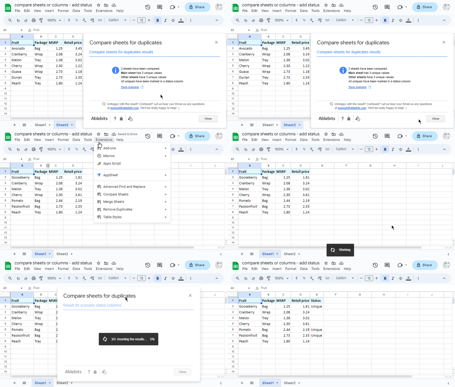
I used the add-on to find the rows from Sheet1 that are absent from Sheet2 (and vice versa) based on Fruit and MSRP columns:

Then I saved my settings into one scenario. Now I can quickly run them without going through all steps again whenever records in my tables change. I just need to start that scenario from the Google Sheets menu:
If you're feeling excited about this tool, go ahead and click that image below to install it from the Google Workspace Marketplace. You'll notice how much time it saves you :)
This help page will gently guide you in case you're stuck on any step.
Compare sheets cell by cell
This on is also part of the Compare Sheets collection. It will compare your Google Sheets for differences. Whether you have two or more tables, it will check them all cell by cell and create one thorough report with differences from all sheets grouped accordingly.
Here's an example of the same two tables. The add-on creates one report with not only different cells (marked with yellow) but also unique rows (marked with red and blue):

Video: How to work with the comparison report
To look at the report and all its parts closely, feel free to read this tutorial or watch this demo video:
Try both add-ons for yourself and notice how much time they save you. :)
Compare data in two Google Sheets and fetch missing records
Comparing two Google Sheets for differences and repeats is half the work, but what about missing data? There are special functions for this as well, for example, VLOOKUP. Let's see what you can do.
Find missing data
Example 1
Imagine you have two lists of products (columns A and C in my case, but they can simply be on different sheets). You need to find those presented in the first list but not in the second one. This formula will do the trick:
=ISERROR(VLOOKUP(A2,$C:$C,1,0))
How does the formula work:
- VLOOKUP searches for the product from A2 in the second list. If it's there, the function returns the product name. Or else you will get an #N/A error meaning the value wasn't found in column C.
- ISERROR checks what VLOOKUP returns and shows you TRUE if it's the value and FALSE if it's the error.
Thus, cells with FALSE are what you're looking for. Copy the formula to other cells to check each product from the first list:

Note. If your columns are in different sheets, your formula will reference one of them:
=ISERROR(VLOOKUP(A2,Sheet2!$C:$C,1,0))
Tip. To get by with a one-cell formula, it should be an array one. Such formula will automatically fill all cells with results:
=ArrayFormula(ISERROR(VLOOKUP(A2:A10,$C:$C,1,0)))
Example 2
Another smart way would be to count all appearances of the product from A2 in column C:
=IF(COUNTIF($C:$C, $A2)=0, "Not found", "")
If there's absolutely nothing to count, the IF function will mark cells with Not found. Other cells will remain empty:

Example 3
Where there's VLOOKUP, there's MATCH. You know that, right? ;) Here's the formula to match products rather than count:
=IF(ISERROR(MATCH($A2,$C:$C,0)),"Not found","")
Tip. Feel free to specify the exact range of the second column if it remains the same:
=IF(ISERROR(MATCH($A2,$C2:$C28,0)),"Not found","")
Pull matching data
Example 1
Your task may be a bit fancier: you may need to pull all missing information for the records common for both tables, for example, update prices. If so, you'll need to wrap MATCH in INDEX:
=INDEX($E:$E,MATCH($A2,$D:$D,0))
The formula compares fruits in column A with fruits in column D. For everything found, it pulls the prices from column E to column B.

Example 2
As you may have guessed, another example would use the Google Sheets VLOOKUP function that we described some time ago.
Yet, there are a few more instruments for the job. We described them all in our blog as well:
Merge sheets using the add-on
If you're tired of formulas, you can use our Merge Sheets add-on to quickly match and merge two Google sheets.
Alongside its basic purpose to pull the missing data, it can also update existing values and even add non-matching rows. You can see all changes in colour or in a status column that can be filtered.
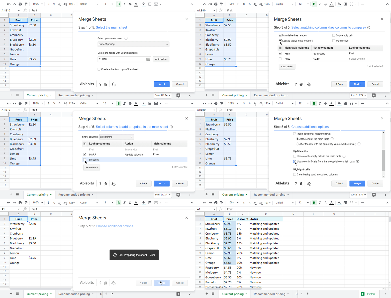
The 2.0 version of Merge Sheets will merge not just 2 tables (one main with one lookup) but multiple sheets in a row (one main with several lookups). The data from the lookup sheets will be added to your main one by one: as you added them in the add-on. Lots of additional options will make your merge as comprehensive as you need.
Video: How to use Merge Sheets add-on for Google Sheets
Check out this video about the Merge Sheets add-on. Though it features just 2 sheets, it paints a clear picture of the add-on possibilities:
Conditional formatting to compare data in two Google Sheets
There's one more standard way Google offers to compare your data – by colouring matches and/or differences via conditional formatting. This method makes all records you're looking for stand out instantly. Your job here is to create a rule with a formula and apply it to the correct data range.
Highlight duplicates in two sheets or columns
Let's compare two columns in Google Sheets for matches and colour only those cells in column A that tally with cells in the same row in column C:
- Select the range with records to color (A2:A10 for me).
- Go to Format > Conditional formatting in the spreadsheet menu.
- Enter a simple formula to the rule:
=A2=C2 - Pick the color to highlight cells.
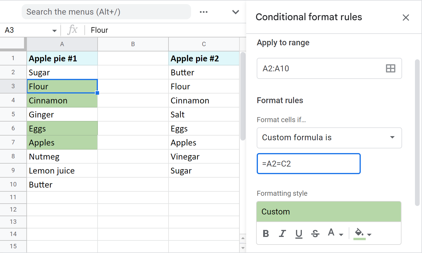
Tip. If your columns change in size constantly and you want the rule to consider all new entries, apply it to the entire column (A2:A, assuming the data to compare starts from A2) and modify the formula like this:
=AND(A2=C2,ISBLANK(A2)=FALSE)
This will process entire columns and ignore empty cells.
Note. To compare data from two different sheets, you'll have to make other adjustments to the formula. You see, conditional formatting in Google Sheets doesn't support cross-sheet references. However, you can access other sheets indirectly:
=A2=INDIRECT("Sheet2!C2:C")
In this case, please specify the range to apply the rule to – A2:A10.
Compare two Google sheets and columns for differences
To highlight records that don't match cells on the same row in another column, the drill is the same as above. You select the range and create a conditional formatting rule. However, the formula here differs:
=A2<>C2
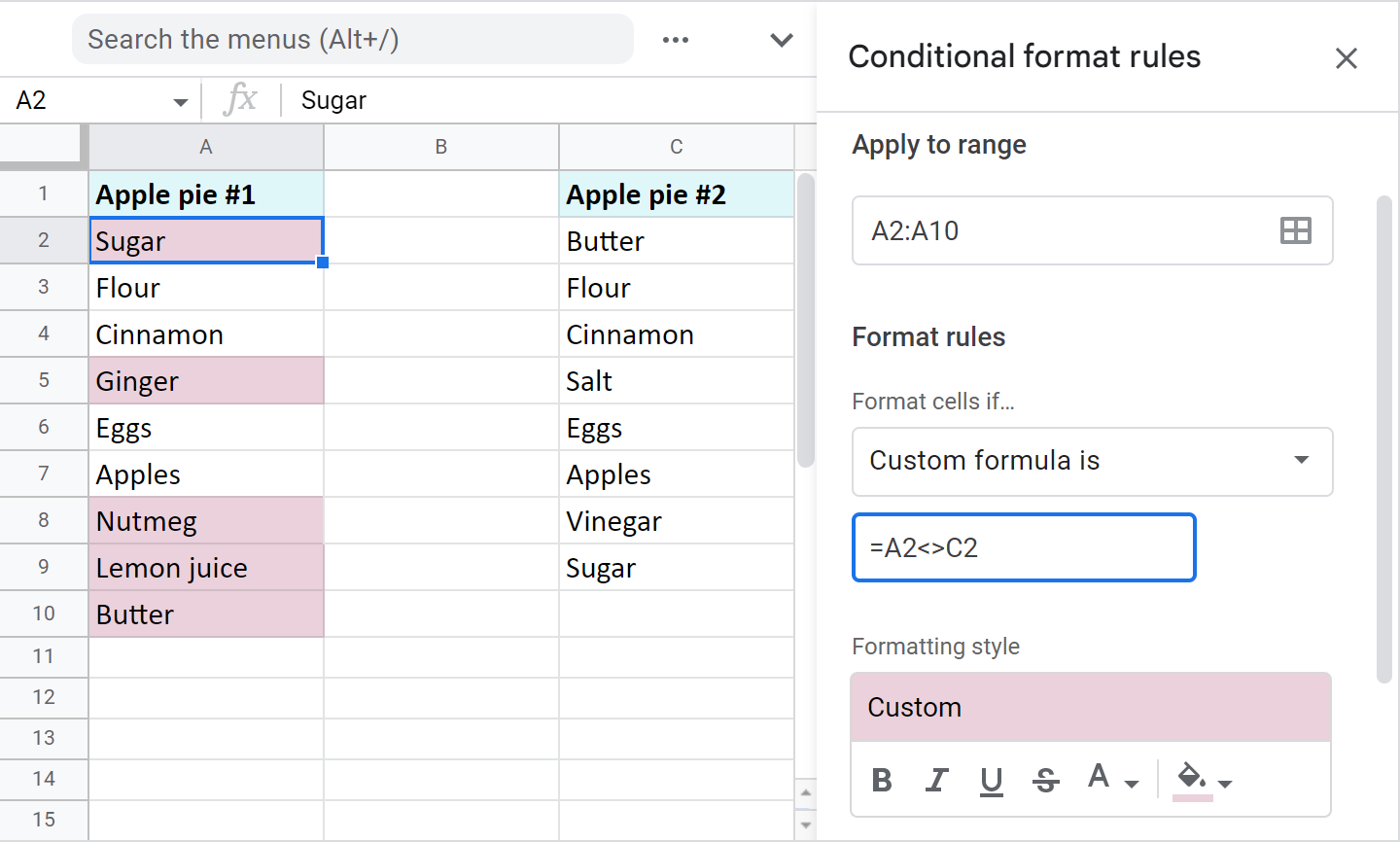
Again, modify the formula to make the rule dynamic (have it consider all newly added values in these columns):
=AND(A2=C2,ISBLANK(A2)=FALSE)
And use the indirect reference to another sheet if the column to compare with is there:
=A2<>INDIRECT("Sheet1!C2:C")
Note. Don't forget to specify the range to apply the rule to – A2:A10.
Compare two lists and highlight records in both of them
Of course, it's more likely the same records in your columns will be scattered. The value in A2 in one column will not necessarily be on the second row of another column. In fact, it may appear much later. Clearly, this requires another method of searching for the items.
Example 1. Compare two columns in Google Sheets and highlight differences (uniques)
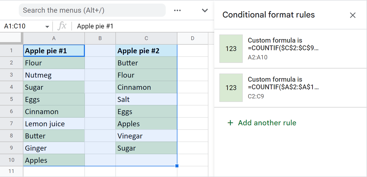
To highlight unique values in each list, you must create two conditional formatting rules for each column.
Color column A: =COUNTIF($C$2:$C$9,$A2)=0
Color column C: =COUNTIF($A$2:$A$10,$C2)=0
Here are the uniques I've got:

Example 2. Find and highlight duplicates in two columns in Google Sheets
You can colour common values after slight modifications in both formulas from the previous example. Just make the formula count everything greater than zero.
Color dupes between columns in A only: =COUNTIF($C$2:$C$9,$A2)>0
Color dupes between columns in C only: =COUNTIF($A$2:$A$10,$C2)>0
Tip. Find many more formula examples to highlight duplicates in Google Sheets in this tutorial.
3 quickest ways to match columns and highlight records
Conditional formatting can be tricky sometimes: you may accidentally create a few rules over the same range or apply colors manually over cells with rules. Also, you have to keep an eye on all ranges: the ones you highlight via rules and those you use in the rules themselves. All of these may confuse you a lot if you're not prepared and not sure where to look for the problem.
Luckily, our Compare Sheets collection for Google Sheets has 3 user-friendly solutions for you.
Video: What is Compare Sheets collection
Add-on to compare & highlight duplicates or uniques
Compare sheets for duplicates is intuitive enough to help you match different tables within one file or two separate files, and highlight those uniques or dupes that may sneak into your data.
Here's how I highlighted duplicates between just two tables based on Fruit and MSRP columns using the tool:
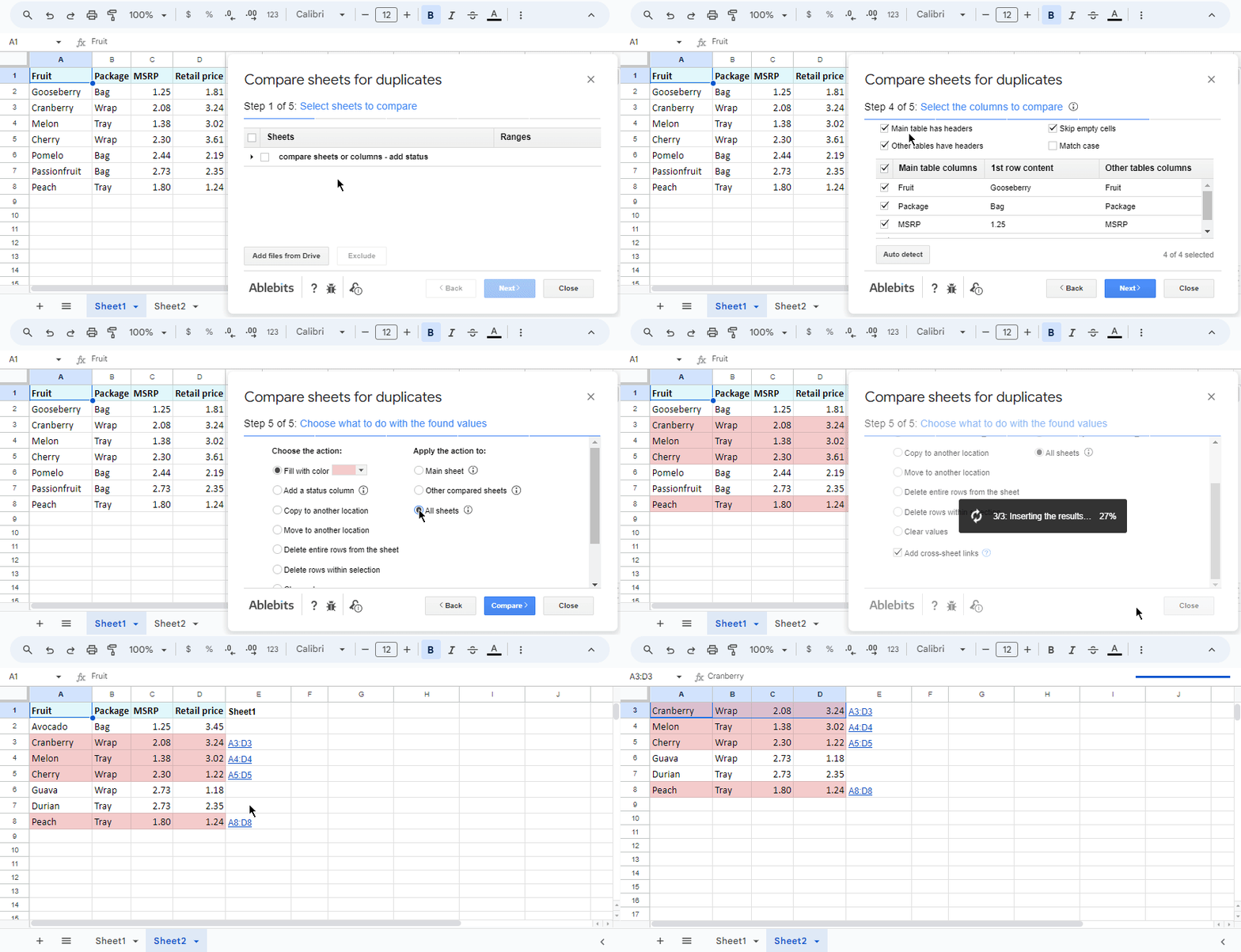
I can also save these settings into a reusable scenario. If the records update, I will call for this scenario in just a click and the add-on will immediately start processing all the data. Thus, I avoid tweaking all those settings over the add-on steps repeatedly. You will see how scenarios work in the example above and in this tutorial.
Add-on to compare Google sheets and highlight differences
Compare sheets cell by cell doesn't fall behind. It sees all differences between two columns or sheets. In fact, it compares as many sheets as you need, even from different files. Usually, one of these tables acts as your main one, and you compare it with others. The add-on highlights differences on those other sheets so you could spot them instantly:

Video: How to use Compare Sheets Cell by Cell add-on
This help page and the demo video below will give you a better idea of how it compares multiple Google sheets for differences:
Compare two columns and color dupes/uniques
This last tool comes in especially helpful for a simpler task: comparing just two columns within one Google tab. Why especially helpful? Because since both columns are on one sheet, going over 5 steps is too much. Hence, there's only one step with all the necessary settings:

This tutorial discusses every option in detail if you'd like to take a look.
And guess what? This tool is also part of the Compare Sheets collection from the Google Workspace Marketplace.
That's right: you get all 3 tools with just one add-on. Give it a go and you won't regret it! (And if you do, let me know why in the comments section!)
Anyways, all these methods are now at your disposal – experiment with them, modify and apply them to your data. If none of the suggestions help your particular task, feel free to discuss your case in the comments down below.
 by
by 
215 comments
Hi
I have a google sheet of students reading levels that are letters. I would like to find the difference between for example e3-d3 to calculate growth. How do I do this? Thanks!
Hi Andrea,
For me to be able to suggest you anything, please share a small sample spreadsheet with us (support@4-bits.com) with 2 sheets: your source data and the result you expect to get. I kindly ask you to shorten the tables to 10-20 rows.
Note. We keep that email for file sharing only and don't monitor its Inbox. Please do not email there. Once you share the file, just confirm by replying here.
Hi,
I have a team of 14 people. I have to manually enter their name and email addresses in col3 and col4. Is there a way I can enter their name and their email address comes up automatically in the next col?
Eg: Name Email address
ABC Abc@gmail.com
DEF Def@gmail.com
ABC Abc@gmail.com
Hi Midnite,
Suppose you enter names to column A on Sheet1, and you need to have emails in column B, same Sheet1.
To do this, first, list each and every name and its corresponding email on a separate sheet, for example, Sheet2, in columns A and B respectively.
Then, build a VLOOKUP formula like this in column B, Sheet1:
=VLOOKUP($A2,Sheet2!$A$2:$B$15,2)
Once you enter the name from the list to A2, B2 will be automatically filled with the needed email.
Hello
I need to identify the different attendees year on year. Column A is all the attendees in 2017, column B is all the attendees in 2018. I want a list of persons who came in 2017 and not in 2018 and also who came in 2018 but not in 2017.
Doing this manually is taking a great deal of time and is not reliably accurate.
Thanks for your help
Tony
Hello Tony,
Please try the solutions from the following paragraphs of the article above:
Find missing data
Compare two lists and highlight records in both of them
To automate the task even more, you can try a special comparing tool as described here.
Hi, is it possible to compare 2 pivot table and calculate the sum of both pivot table?
Pivot table 1 is tab IN, pivot table 2 is tab OUT. I need to know the sum of person A IN minus the sum of person A in tab OUT. So that I can know the actual sum of person A in certain date.
Hi Wyatt,
Yes, you just need to reference the tabs with your pivot tables in your formulas.
Hey, thanks for posting. Rly need help here.
I need a function for:
If the content of Column B in sheet 1 matches the content of Column B in sheet 2, then answer YES in column E in the same row that column b sheet 1 is in.
Help!!!
Hi Charlie,
Assuming you compare cells from B2:B10, try this formula in column E, Sheet 1:
=ArrayFormula(IF(Sheet1!B2:B10=Sheet2!B2:B10,"YES",""))
This case is described in this part of the article in detail.
Hi i wanted to know which formula shall I use when the case is: is to find if the Email id in Column B in sheet A is Equal to Email id In Column D Sheet B then Copy the Data of Column C i.e Mobile Number in Sheet A to Column C in Sheet B.
Hi Gaurav,
There are a few ways to match records and pull missing information. All of them are described in this part of the post.
Hi, our company needs to update the prices of its stock monthly as we get price updates from them every month. Is there a way to compare an old list of prices with the updated list and then highlight which ones have changed? At the moment we are having to do it by eye. Thank you.
Hi,
Our Compare columns or sheets may be able to help. It will compare your price lists and color differences for you. You can try out the tool for 30 days for free.
Hello,
I have a Google Form people filled out, in total I need about 220 responses.
People have filled out their e-mail adresses and I want to check if everyone I sent it too actually filled it in.
If not, I can remind them to fill it out.
Is there a way I can crossreference the filled out email adresses with my imported list of e-mail adresses I sent the form too?
For example, I sent the email too hello1@gmail.com and hello2@gmail.com
I want to filter out which one hasnt filled out the form yet, so I can remind them.
Not sure if you will read it, but I'll give it a shot.
Hello Joey,
You can export the sheet of all emails to the file that people fill out. Then use our tool to quickly compare columns with emails for unique addresses. It is described in the last paragraph above.
If you don't want to use the tool, please look through this paragraph for other workarounds.
I am scraping data from the web in two columns and want to find the common values between the two columns (ie duplicates) and put them on the thrid column.
As I am scraping the data, I do not know how many cells I will have at any given time.
Any help appreciated!
Hello Nickolas,
If you want to use formulas, you need to know the exact number of duplicates because formulas won't supply you with additional rows.
So I'd advise you to try our Compare two sheets or columns tool. It will copy/move duplicate values to any place you select. If the sheet is short on rows, the tool will insert them along with the dupes.
Hey, you seem super knowledgable and this is about as close as I've come to a solution for my problem.
I'm putting together a data set, which is basically a list of countries in row A, and I want to add data in form of entire columns - typically two columns where one is the list of countries and the other one is the data input. The issue is that some lists don't include all countries, for which I'd like to leave an empty row in that specific column of data.
Here's how I want it to look:
https://cdn3.imggmi.com/uploads/2019/10/22/3e9f91f0e882d2296a8f2b3e0cf40c59-full.png
On the right how it ends up, compared to my full list of countries:
https://cdn3.imggmi.com/uploads/2019/10/22/37545ca2a98a32471307627200bdeb09-full.png
I'm very greatful for any help of redirection towards a solution!
Hello Viking,
If I get it correctly, it looks like our Merge Sheets can help you. It pulls the related data from one table to another and adds missing rows with the rest of the countries.
In the end, you can simply sort the table by countries A>Z.
You can test the tool for 30 days for free to see if it suits your needs.
You're absolutely correct, Merge Sheets helped immensely and I appreciate you taking the time to help me out!
Please, i need a formula to remove duplicates from a large data of name and phone number from two different columns. Thanks
Hello Olumose,
I'm afraid the formula won't remove duplicates. You can use formulas to copy all unique or duplicate info to someplace else. Or create conditional formatting rules to colour duplicates where they reside.
However, there's a special tool that may help get rid of dupes. It offers 30 days of free use, so feel free to try it on your data:
https://workspace.google.com/marketplace/app/remove_duplicates/347814268012
Hi! This is very helpful!
I've used =ISERROR(VLOOKUP(C3,$G:$G,1,0)), and it gives me a FALSE if the C and G columns have the same name, and TRUE if it only exists in C.
Is there a way to list the True values in a single, tight column, excluding the False?
My project is a list of clients that need a specific task. If it has been accomplished, then the name is in G and C. G is all clients, C is a subset of those clients with the task completed. So, I'm looking for a list of clients who need the task. Thanks in advance,
Alex
Hi Alexander,
I'm sorry but your task is not entirely clear. Please consider sharing a small sample with us (support@4-bits.com) with your source data and the result you expect to get. I kindly ask you to shorten the table to 10-20 rows.
Since we keep that email for file-sharing only, once you share the file, please confirm by replying here. Thank you.
In the meantime, you can check our blog post devoted to Google Sheets VLOOKUP function. Perhaps, it'll help.
I am trying to test for conditions in two different columns and count the number of times the condition is true in both columns.
For instance if the Value is "Closed" in column F and the Value is "M" in column K then count that row.
Todd,
this formula should help:
=COUNTIFS(F:F,"Closed",K:K,"M")
For more info please look through these blog post and comments.
Hi Natalia, I am hoping you will help me with a way to identify the common row fields from the two columns. They may not be in the same row and I want to identify the common in both columns appearing in anywhere in the two columns. All the fields in the individual columns are unique. Thanks for the opportunity to ask you this question.
Hi Sam,
Please look through this part of the article. It explains how to compare two columns for differences or duplicates no matter their position in columns.
I am trying to compare/list duplicates taken from a calendar.
Columns A and B are where people list their names and holiday dates. These columns got pretty bug quite quickly. To simplify looking for any available dates that you may want off I have created a drop down in J14 where you can select the month and which pulls the calendar for that month into cells J16:P21.
I have taken dates from the list in column B and highlight the corresponding dates in the calendar in J16:P21.
But, I want to list the people and the dates which they have booked off underneath the calendar.
To recap.... compare dates from column B2:B to the calendar J16:P21 and list duplicates and the corresponding name from column A2:A
Hello David,
For us to be able to help you better, please share a small sample spreadsheet with us (support@4-bits.com) with your source data and the result you expect to get. I kindly ask you to shorten the table to 10-20 rows.
Since we keep that email for file-sharing only, once you share the file, please confirm by replying here. Thank you.
Hi,
I have two separate Google Sheets, I need to take information from one sheet to the other. Using INDEX, MATCH how would I pull information over from one sheet to the other? MATCH("X",Sheet #2 URL, 0) doesn't seem to work
Thanks
Hi Patrick,
To do a v-lookup from another Google spreadsheet, you need to add IMPORTRANGE to your formula. Svetlana has provided the example here:
https://www.ablebits.com/office-addins-blog/vlookup-google-sheets-example/#comment-321671
Hey Guys!
I'm having trouble doing this for two lists of names from a party. I have tried so many equations but still having trouble.
For example, in one column I have the full list of invited guests and then in column B I have all the people who have paid. I am trying to find who hasn't paid for their ticket to the party. Can someone help me out?
Cheers!
Hey Xavier,
It looks like you need to find those names in column A that are not in column B. This point of the article offers a short formula to solve this:
https://www.ablebits.com/office-addins-blog/google-sheets-compare-two-sheets-columns/#find-missing-data
If you'd rather use colours, please read through this paragraph:
https://www.ablebits.com/office-addins-blog/google-sheets-compare-two-sheets-columns/#highlight-both-lists
Make sure your names are written identically and there are no extra spaces or other chars in them.
I have two sheets of color names. in sheet one I have all the colors organized under their primary colors. I want to look for colors in column A of Sheet2 inside the table in Sheet1 and return in column B of Sheet2 the title of the column it was found in Sheet1. if there are multiple found then all in one cell separated with comma and no space. thanks
Hello Maae,
For us to be able to help you, please share a small sample spreadsheet with us (support@apps4gs.com) with 3 sheets: where 1st and 2nd are your sheets with colors and 3d is the result you need to get. I kindly ask you to shorten the tables to 10-20 rows.
Note. We keep that Google account for file sharing only, please do not email there. Once you share the file, just confirm by replying here.
We'll look into your task and see if our software can help.
Hi
I you have a user database with all names in the SHEET1 A:A but in SHEET2!A:A you only have some of the names, and same with SHEET3A:A and SHEET4!A:A
What if In SHEET1 you want the B:B collum to refference to what other sheet has the same name.
So if the First name in The Sheet 1 list is «John B» And «John B» is also the 13th name in the SHEET3. How do I get SHEET!B1 to say SHEET3 when SHEET!A1 says «John B» ?
If that makes any sence? What would the formula be in B1 (and dragged down for the rest of the sheet)
Hi Christian,
If I get your task correctly, this formula will help:
=IF(COUNTIF(Sheet3!$A:$A,A1)>0,"Sheet3","")
If you'd like to check in all 3 sheets at the same time and return the corresponding sheet name, try this one instead:
=IF(COUNTIF(Sheet2!$A:$A,A1)>0,"Sheet2",IF(COUNTIF(Sheet3!$A:$A,A1)>0,"Sheet3",IF(COUNTIF(Sheet4!$A:$A,A1)>0,"Sheet4","")))
Keep in mind that once the formula finds the value in Sheet2, it won't look in other sheets, it will return "Sheet2" right away. If the searched entry is absent from all three sheets, cells with formula will remain blank.
Hi everyone,
Can somone please help me with which formula to use:
If Value in Column B is Column B minus Column A equal or greater than 2, then highlight Column B. So for example:
Column A Column B
100 103 = 103 is highlighted
100 101 = 101 is not highlighted
Thanks to whoever can answer this.
Hi Joy,
You need to create a conditional formatting rule with the following formula:
=($B2-$A2)>=2
Hi,
I have to separate Google Spreadsheets. I need to make sure that they are identical. How can I compare the data between two separate spreadsheets?
Thank you,
Violet
Hi Violet,
To reference another spreadsheet, you need to use the IMPORTRANGE function.
Thus, your formula to compare two Google Sheets for differences may look like this:
=IF(Sheet1!A1<>IMPORTRANGE("link_to_your_2nd_spreadsheet","Sheet1!A1"),Sheet1!A1&" | "&IMPORTRANGE("link_to_your_2nd_spreadsheet","Sheet1!A1"),"")