Keeping track of all external references in a workbook can be challenging. This tutorial will teach you a few useful techniques to find links to external sources in Excel formulas, objects and charts and shows how to break external links.
When you want to pull data from one file to another, the fastest way is to refer to the source workbook. Such external links, or external references, are a very common practice in Excel. After completing a particular task, however, you may want to find and probably break those links. Astonishingly, there is no quick way to locate all links in a workbook at once. Depending on exactly where the references are located - in formulas, defined names, objects, or charts - you will have you use different methods.
How to find cells with external links in Excel
External links in cells are the most common case. They are also the easiest to find and remove. For this, you can utilize the Excel Find feature:
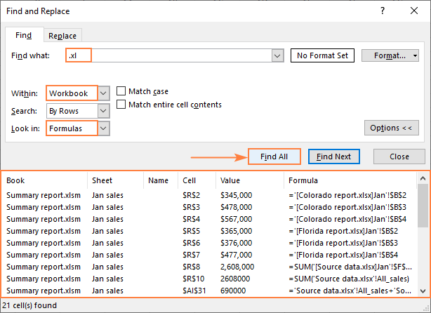
- In your worksheet, press Ctrl + F to open the Find and Replace dialog.
- Click the Options button.
- In the Find what box, type .xl. This way, you will search for all possible Excel file formats including .xls (older workbooks) .xlsx (modern workbooks) .xlsm (macro-enabled workbooks), etc.
- In the Within box, select either Workbook to search in all tabs or Sheet to look in the current worksheet only.
- In the Look in box, choose Formulas.
- Click the Find All button.
That's it! You've got a list of cells that have any external references in them.

And these useful tips will help you manage the results:
- To select a cell that contains an external link, click the cell address in the Cell
- To group the found links the way you want, click the corresponding column header, for example, Sheet or Formula.
- To select all cells with external references, place the cursor anywhere within the results and press Ctrl + A. This will select both the results in the Find and Replace dialog box and the cells in the workbook.
Note. With Find and Replace you can only identify external links in cells. If you've removed all external references from formulas but Excel still says there are links to external workbooks, then check other possible locations discussed below.
How to find links in Excel named ranges (defined names)
Excel pros often name ranges and individual cells to make their formulas easier to write, read, and understand. Data validation drop-down lists are also easier to create with named ranges, which in turn may refer to outside data. To take care of such cases, check for external links in Excel names:
- On the Formulas tab, in the Defined Names group, click Name Manager or press the Ctrl + F3 key combination.
- In the list of names, check the Refers Tocolumn for external links. References to other workbooks are enclosed in square brackets like [Source_data.xlsx].

How to identify external links in Excel objects
If you've linked objects such as shapes, text boxes, WordArt and the like to other Excel files, then you can use the Go To Special feature to locate such links:
- On the Hometab, in the Formats group, click Find & Select > Go to Special. Or press F5 to open for the Go To dialog, and then click Special… .
- In the Go To Special dialog box, select Objects and click OK. This will select all objects on the active sheet.

- Press the Tab key to cycle through the selected objects and check each individual object for references to other workbooks.
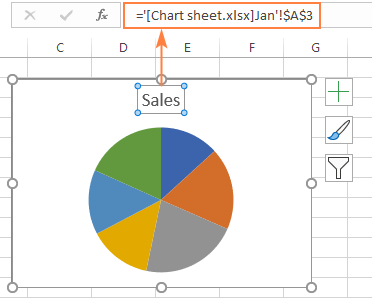
If an object is linked to a specific cell, you can see an external reference in the formula bar:

If an object is linked to a file, then hover over the object with your mouse to see where it points to:

Note. If an object is linked to a whole file rather than an individual cell, such link cannot be broken by using the Edit Links feature. To remove the link, right-click the object and select Remove link from the context menu.
How to find links to other files in Excel charts
In case external links are used in a chart title or data series, you can locate them in this way:
- On the graph, click the chart title or data series you wish to check.
- In the formula bar, look for a reference to another Excel file.
External reference in chart title:

External link in chart data series:

If your chart contains several data series, you can quickly move between them in this way:
- Select the target chart.
- Go to the Format tab > Current Selection group, click the arrow next to the Chart Elements box, and select the data series of interest.

How to find external links in Pivot Tables
Most often a PivotTable is created using the data in the same workbook. But sometimes, the source data resides in an outside file. To find the exact location of your PivotTable's source data, perform these steps:
- Click any cell within the Pivot Table.
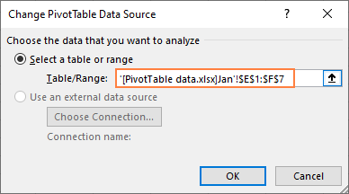
- On the PivotTable Analyze tab, in the Data group, click the Change Data Source button.

- In the dialog box that appears, check the data source in the Table/Range box to see whether it is linked externally.

How to enable links to external workbooks in Excel
When you open a workbook with links to other files for the first time, Excel shows a security warning informing you that the file contains links to external data. To allow the links to update, simply click the Enable Content button.
![]()
On subsequent openings of the same file, you will be presented with the following prompt asking if you want to update the links. If you trust the linked documents and want to pull the latest data, click Update.

Control the security prompt about updating links
By default, Excel asks whether or not to update external references every time you open a workbook. However, you can control whether the message appears and whether the links are updated or not.
- On the Datatab, in the Queries & Connections group, click Edit Links.
- In the lower-left corner of the Edit Links dialog box, click Startup Prompt….

- In the Startup Prompt dialog box, choose the option that works best for you:
- Let users choose to display the alert or not (default).
- Don't display the alert and don't update automatic links - it makes sense to choose this option when you are sharing a workbook with other people who do not have access to the source files.
- Don't display the alert and update links - you can choose this setting when you completely trust the sources.

Change security setting for external links
You can also set links to other files to be updated automatically in a particular workbook without getting a security warning by changing the Trust Center security settings:
- In the target workbook, click the File tab > Options.
- In the Excel Options dialog box, click Trust Center > Trust Center Settings.

- In the Trust Center dialog box, click External Content, and then select Enable automatic update for all Workbook Links under Security settings for Workbook Links.
With this option turned on, Excel will update all links to external sources in the current workbook automatically without showing you any warnings or prompts.

Please note that automatic updating of links to unknown files can be harmful and therefore is not recommended. Enable it only when you are 100% confident in the security of the outside data. Or, turn on this option temporarily, and then return to the default Prompt user on automatic update for Workbook Links setting.
Note. Regardless which option you choose, Excel will still display the below prompt if the workbook contains invalid or broken links.

How to break external links in Excel
In Excel, breaking a link to another workbook means replacing an external reference with its current value.
For example, if you break the following external reference, it will be replaced with the value that is currently in cell A1 on the Jan sheet in the Source data workbook:
='[Source data.xlsx]Jan'!$A$1
If you break an external link in the below formula, the formula will be changed to its calculated value, whatever it is:
=SUM('[Source data.xlsx]Jan'!A2:A7)
Note. Because breaking links is the action that cannot be undone, it may be wise to save a backup copy of your workbook first.
To break external links in Excel, this is what you need to do:
- On the Data tab, in the Queries &Connections group, click the Edit Links button.
If this button is greyed out, that means there is no linked data in your workbook.
- In the Edit Links dialog box, select the links that you want to break.
- To select multiple links, click on each one individually while holding down the Ctrl key.
- To select all links, press the Ctrl + A shortcut.
- Click the Break Link button.


Note. Under ideal circumstances, this feature should remove all external links in a workbook. Unfortunately, we do not live in a perfect world :( Some links to outside data, e.g. external source data in Pivot Tables, are not shown in the Edit Links dialog while others cannot be broken. If the Edit Links button is grayed out in your workbook but you are still getting a prompt about external data, then you will have to check each possible place where external references may be lurking (such as objects, charts, etc.) and change or remove the links manually.
Get a list of all external links in a workbook
To get a list of all external sources that your workbook refers to, you can use one of the following methods.
Traditional approach
The conventional way to check links in Excel is by using the Edit Links feature: Data tab > Queries & Connections group > Edit Links.
This will display the following information:
- Source - the name of the linked file
- Type - the link type: a workbook or worksheet
- Update - whether the link updates automatically or manually
- Status - the status of the link such as OK, Source is Open, Warning, Unknown, etc. To get the most recent info, click the Check Status button on the right.

Very quick and straightforward, this method is not very convenient though. To see the location of the source file, you need to click each link, one at a time.
Dynamic arrays and Excel 4.0 macros.
A very cute trick suggested by Bob Ulmas in his book "This isn't Excel, it's Magic!" can help you retrieve the locations of all source files in one go. The solution combines the recently introduced dynamic arrays with the good old Excel 4.0 macros.
To generate a list of all external references in a given workbook, this is what you need to do:
Step 1. Create a new name that references the macro
To be able to use a built-in Excel 4.0 macro in a formula, you need to create a name referencing the macro. Here's how:
- On the Formulas tab, in the Defined Names group, click Name Manager. Or simply press the Ctrl + F3 shortcut.
- In the Name Manager dialog window, click the New…
- In the New Name dialog window, type some meaningful name, say GetLinks, in the Name box and the following formula in the Refers to box:
=LINKS() - Click OK.

For more detailed instructions, please see How to create a name in Excel.
Step 2. Use the newly create name in a formula
Now that you have a name that references the macro, you just need to put the name in a formula. Depending on your Excel version, the formula will take a different form.
In Excel 365:
In the topmost cell of the destination range, enter this formula:
=TRANSPOSE(GetLinks)
GetLinks (or any other name that you utilized for referencing the macro) returns a horizontal spill range of all the external links in the workbook. The TRANSPOSE function rotates rows to columns and outputs a vertical list that is easier to read.

To arrange the list in alphabetical order, put the above formula inside the SORT function:
=SORT(TRANSPOSE(GetLinks))
Please remember that this solution only works in Excel 365 that has a new calculation engine supporting dynamic arrays.
In Excel 2019 - 2007:
In pre-dynamic versions of Excel, use the GetLinks name for the array argument of the classic INDEX function. To make the solution more user-friendly, you can wrap the construction in IFERROR to take care of situations when the formula is copied to more cells than there are external references in your workbook:
=IFERROR(INDEX(GetLinks, ROW(A1)), "")
The formula goes to the first cell (A2), and then you drag it down to the below cells:

Important notes:
- Because this solution uses macros, the file must be saved as a Macro-Enabled Workbook (.xlsm).
- Excel macros do not execute nor update automatically. To refresh a list of links, press the Ctrl + Alt + F9 keys shortcut, which recalculates all formulas in all open workbooks.
VBA macro to get a list of external links
If you have nothing against using macros in your worksheets, the following VBA code can find and list down all links to external sources in a workbook automatically:
To add the code to your workbook, do the following:
- Press Alt + F11 to open the Visual Basic Editor.
- On the left pane, right-click your workbook, and then click Insert > Module.
- Paste the above code in the Code window.
For the detailed steps, please see How to insert VBA code in Excel.
To run the macro, press either Alt + F8 in a workbook or F5 in the VBA Editor.
For more information, please see How to run macro in Excel.
As the result, you will get a list of external sources in a new sheet:

Find cells with external links using VBA
If your goal is to get a complete list of all external references in a workbook including the addresses of the cells containing the links, the following code can be helpful. Here, we utilize the LinkSources method to get all source workbooks and the LinkInfo method to identify their status. The status of a link is determined as described on this page:
https://docs.microsoft.com/en-us/office/vba/api/excel.xllinkstatus
The results are output in a new worksheet named All Links report. Column B contains hyperlinks to the cells with outside links.

To make use of the code straight away, you can download our sample workbook at the end of the post. The workbook contains the above code as well as the detailed step-by-step instructions on how to run it.
Find all external links in a workbook in a click
Reading the previous examples, perhaps you were wondering why simple things need to be made so complicated. We also asked that question to ourselves… and implemented a one-click solution for this task.
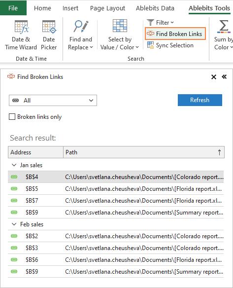
With Ultimate Suite installed in your Excel, finding all links in a workbook takes a single click on the Find Links button:

By default, the tool looks for all links: internal, external and web pages. To display only external references, select this option in the drop-down list and click the Refresh button.

To show only broken links, just put a tick in the corresponding check box.
To get to a cell that references external data, click the cell address on the pane.
Simple things should be kept simple! :)
That's how to find links to external sources in Excel. I thank you for reading and hope to see you on our blog next week!
Available downloads:
Ultimate Suite 14-day fully-functional version (.exe file)
VBA codes to find external links (.xlsm)
 by
by
4 comments
Ctrl+F3 option worked for me to fix this annoying error. Thanks!
Thank you!!! The best solution to my problem unable to find the error to the unfound link mentioned. Indeed it's ANNOYING error.
One item additional item to look for:
Cells with data validation (the list it refers back to may be an external link)
If copied and pasted from another workbook this can be unintentionally carried over.
Thx a lot !!!! This is the only spot where any macro / search tool / go to tool cant go. And obviously that was where my link was.