This next bit of our operations with text in spreadsheets is devoted to extraction. Find out ways to extract various data — text, characters, numbers, URLs, email addresses, date & time, etc. — from various positions in multiple Google Sheets cells at once.
Google Sheets formulas to extract text and numbers from strings
Formulas in Google Sheets are everything. While some combos add text & numbers and remove various characters, some of them also extract text, numbers, separate characters, etc.
The easiest functions to deal with when you're about to take out data from Google Sheets cells are LEFT, RIGHT, and MID. They get any data by position.
Extract data from the beginning of cells in Google Sheets
You can easily pull out the first N characters using the LEFT function:
- string is the text where you want to extract data from.
- number_of_characters is the number of characters to take out starting from the left.
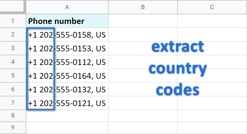
Here's the simplest example: let's take out the country codes from the phone numbers:

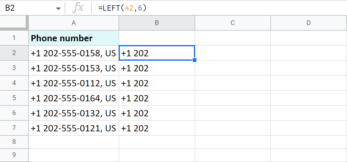
As you can see, country codes take 6 symbols at the beginning of cells, so the formula you need is:
=LEFT(A2,6)

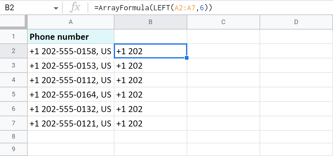
Tip. ArrayFormula will make it possible to get 6 characters from the entire range at once:
=ArrayFormula(LEFT(A2:A7,6))

Extract data from the end of cells in Google Sheets
To pull out the last N characters from cells, use the RIGHT function instead:
- string is still the text (or a cell reference) to extract data from.
- number_of_characters is also the number of characters to take from the right.
Let's get those country names from the same phone numbers:

They take only 2 characters and that's exactly what I mention in the formula:
=RIGHT(A2,2)

Tip. ArrayFormula will also help you extract data from the end of all Google Sheets cells at once:
=ArrayFormula(RIGHT(A2:A7,2))

Extract data from the middle of cells in Google Sheets
If there are functions to extract data from the beginning and the end of cells, there must be a function to extract data from the middle as well. And yes — there is one.
It's called MID:
- string — the text where you want to take out the middle part from.
- starting_at — the position of the character from which you want to start getting the data.
- extract_length — the number of characters you need to pull out.
By the example of the same phone numbers, let's find the phone numbers themselves without their country codes and country abbreviation:

As the country codes end with the 6th character and the 7th is the dash, I will pull numbers starting from the 8th digit. And I'll get 8 digits in total:
=MID(A2,8,8)

Tip. Changing one cell to the entire range and wrapping it in ArrayFormula will provide you with the result for each cell at once:
=ArrayFormula(MID(A2:A7,8,8))

Extract data before a certain text — LEFT+SEARCH
Sometimes extracting text by position (as shown above) is not an option. The required strings may reside in any part of your cells and consist of a different number of characters forcing you to create different formulas for each cell.
But Google Sheets wouldn't be Google Sheets if it didn't have other functions that would help to extract text from strings.
Whenever you want to extract data that precedes a certain text, use LEFT + SEARCH:
- LEFT is used to return a certain number of characters from the beginning of cells (from their left)
- SEARCH looks for certain characters/strings and gets their position.
Combine these — and LEFT will return the number of characters suggested by SEARCH.
Here's an example: how do you extract textual codes before each 'ea'?

This is the formula that will help you in similar cases:
=LEFT(A2,SEARCH("ea",A2)-1)

Here's what happens in the formula:
- SEARCH("ea",A2) looks for 'ea' in A2 and returns the position where that 'ea' starts for each cell — 10.
- So 10th position is where 'e' resides. But since I want everything right before 'ea', I need to subtract 1 from that position. Otherwise, 'e' will be returned as well. So I get 9 eventually.
- LEFT looks at A2 and gets the first 9 characters.
Extract data after the text
There are also means to get everything after a certain text string. But this time, RIGHT won't help. Instead, REGEXREPLACE takes its turn.
Tip. REGEXREPLACE uses regular expressions. If you're not ready to deal with them, there's a much easier solution described below.
- text is a string or a cell where you want to make changes
- regular_expression is the combination of characters that stands for a part of the text that you're looking for
- replacement is whatever you want to get instead of that text
So, how do you use it to extract data after a certain text — 'ea' in my example?

Easy — using this formula:
=REGEXREPLACE(A2,"(.*)ea(.*)","$2")

Let me explain how this formula works exactly:
- A2 is a cell I'm extracting the data from.
- "(.*)ea(.*)" is my regular expression (or you can call it a mask). I look for 'ea' and put all other characters into brackets. There are 2 groups of characters — everything before 'ea' is the first group (.*) and everything after 'ea' is the second one (.*). The entire mask itself is put to double-quotes.
- "$2" is what I want to get — the second group (hence its number 2) from the previous argument.
Tip. All characters used in regular expressions are collected on this special page.
Extract numbers from Google Sheets cells
What if you want to extract only numbers when their position and whatever goes before & after doesn't matter?
Masks (a.k.a. regular expressions) will also help. In fact, I'll take the same REGEXREPLACE function and change the regular expression:
=REGEXREPLACE(A2,"[^[:digit:]]", "")

- A2 is a cell where I want to get those numbers from.
- "[^[:digit:]]" is a regular expression that takes everything but digits. That ^caret symbol is what makes an exception for digits.
- "" replaces everything except numeric characters with "nothing". Or, in other words, removes it entirely, leaving only numbers in cells. Or, extracts numbers :)
Tip. The following formula return the same result: extract only digits from cells:
=REGEXREPLACE(A2,"[^0-9]", "")
=REGEXREPLACE(A2,"[^\d]", "")
Extract text ignoring numbers and other characters
In a similar fashion, you can take out only alphabetic data from Google Sheets cells. The contraction for the regular expression that stands for text is called accordingly — alpha:
=REGEXREPLACE(A2,"[^[:alpha:]]", "")

This formula takes everything but letters (A-Z, a-z) and literally replaces it with "nothing". Or, to put it in another way, takes out only letters.
Formula-free ways to extract data from Google Sheets cells
Extract URLs from hyperlinks in Google Sheets
When it comes to extracting links from Google Sheets cells, formulas won't help. There are 3 other ways however to get those links out of cells.
Example 1: Copy link
Hover your mouse over a cell with a hyperlink. You'll see a website preview with 3 settings. Go for Copy link:

Then just paste that URL from the clipboard into an empty cell:

Easy-peasy! Yet, you will have to repeat this for every single cell where you'd like to extract those URLs from as the solution doesn't work for cells in batch:

Tip. To extract links from multiple cells in Google Sheets in one go, use the tool described below.
Example 2: Preview the link (edit), then extract
This one is similar to the method above. When you hover the mouse over the link, click Edit link rather than Copy:

You will get a chance to preview the URL itself and maybe copy its certain part if that's what you're up to:

Once you copy the needed part of the URL, paste it to another cell. Repeat for each Google Sheets cell where you need to extract links from:

Tip. To extract links from multiple cells in Google Sheets at once, use the tool from the next example.
Example 3: Extract links add-on for Google Sheets
If you need to extract multiple URLs from multiple hyperlinks in Google Sheets in one go, this will be an indispensable tool for you.
Extract add-on from the Power Tools collection has all the necessary settings for the job.
You just select the range with all the hyperlinks (you can even select several non-adjacent ranges by holding the Ctrl key), open the Extract links group in Power Tools, tweak the settings and click Extract:

Our Power Tools is perfect to extract other types of data as well. Let me show you.
Extract different types of data using Power Tools add-ons
The Extract tool from Power Tools does exactly what you've come looking for in this article — extracts different types of data from Google Sheets cells.
User-friendly settings
All the cases I've covered above are not just solvable with the add-on. The tool is user-friendly so all you need to do is select the range you want to process and tick off the required checkboxes. No formulas, no regular expressions.
Remember this section of this article with REGEXREPLACE and regular expressions? Here's how simple it is for the add-on:

Extra-options
As you can see, there are some extra options (just checkboxes) that you can quickly turn on/off to get the most precise result:
- Get the strings of the required text case only.
- Pull out all occurrences from each cell and place them in one cell or separate columns.
- Insert a new column with the result to the right of the source data.
- Clear the extracted text from the source data.
Extract different data types
Not only Power Tools extracts data before/after/between certain text strings and the first/last N characters; but it also takes out the following:
- Numbers along with their decimals keeping the decimal/thousands separators intact:

- N characters starting from a certain position in a cell.
- Hyperlinks (text + link), URLs (link), email addresses.
Extract any string of data from everywhere
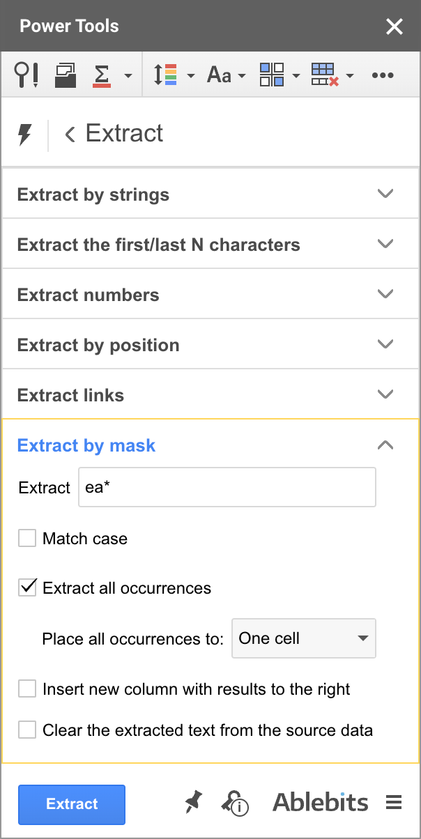
There's also an option to set up your own exact pattern and use it for the extraction. Extract by mask and its wildcard characters — * and ? — do the trick:
- For example, you can bring out everything between the brackets using the following mask: (*)
- Or get those SKUs that have only 5 numbers in their ids: SKU?????
- Or, as I show on the screenshot below, pull everything after each 'ea' in each cell: ea*

Extract date and time from timestamps
As a bonus, there's a smaller tool that will extract date and time from timestamps — it's called Split Date & Time.
Although it was created to split timestamps in the first place, it's perfectly capable of getting one of the desired units individually:

Just select one of the checkboxes depending on what you want to extract — date or time — from timestamps in Google Sheets and hit Split. The required unit will be copied over to a new column (or it will replace the original data if you select the last checkbox as well):

All these Extract tools are part of the Power Tools collection for Google Sheets.
Once you install it to get any data from Google Sheets cells, it's got you covered completely. If not, please leave a comment and we'll help you out :)
 by
by
26 comments
Love this! Thank you so much! I have one question. I am extracting alphanumeric from a cell into another cell when that information is the to the left of a hyphen (-). I used the formula =LEFT(A2,SEARCH("-",A2)-1) The usual cell info in A2 might look like 5588-0023, and therefore it extracts out 5588. However, sometimes the information in column A, might have codes that DO NOT have a hyphen, ex: 6321GKDS, so the formula doesn't know what to do. Is there an "IF" option where by, I can have the formula first try to extract the information that is to the left of the "-", and if there is no "-", then it just extracts the entire contents of that cell. This is what I would like it to do:
1st Priority: Extract info from the left of the "-"
2nd Priority: If there is no "-", then extract the entire content of that cell.
Any help would be appreciated. Thanks!
Thank you for your feedback, Sabrina! :)
The IF function is designed for this task, please read this tutorial.
what if there is more than 1 delimiter? in case more than one "ea"? and i want to target text before the second "ea"
Hello alief,
Do you need to extract everything before the 2nd 'ea' (including the 1st 'ea') or everything between the 1st and the 2nd 'ea' parts?
I Would like to know if this is possible, I want the texts or strings within this character "------------------------------" if its multiple i want that text in adjacent column.
*Date* *Customer* *Project* *Filename* *Turnaround Time*
------------------------------
11/21/2022 20:35 TMB-Readers Digest RD_MARAPR23_Images TP61.jpg
------------------------------
11/21/2022 20:36 TMB-Readers Digest RD_MARAPR23_Images ING_0455.jpg
------------------------------
Hello Anand,
The easiest way is with Power Tools from this part of the blog post:
Hi all,
I want to find the formula ( Query GoogleSheet ) that we can get the number
24307547 from 8949430070120254001.
can you help me ?
Hi Roy,
I'm sorry but I don't see the first number in the second one. Can you explain the logic?
Hello, I've been searching the net for a solution to this issue.
I have data with at column for time that is in the following format, '3d 17h 41m 31s' and I need to change it into numerical form in order to do a leader board.
I think I may need to separate the entries into different columns representing 'Days', 'Hours', 'Minutes' and 'Seconds' and then reconstruct them into a single cell. The formula you've shared has helped, but I really need to know if there is something that I can use to complete the process.
Thanks
Hello Tonya,
So what does your data look like after using the formula? And how would you like it as a result?
Hi Natalia,
Every cell I am working with contain code and names. I need to extract the names. For example:
Cell A1: "Cod.:1 276338Y Jennifer Lawrence"
Cell b2: "Cod.:2 763537U Mike Towers´"
How can I extract the names?
Hello!
Replace the penultimate space with any unique character using the SUBSTITUTE function. Determine the position of this character with SEARCH function. Remove leading characters with the REPLACEB function.
=REPLACEB(A1,1, SEARCH("#", SUBSTITUTE(A1," ","#",len(A1)-len(SUBSTITUTE(A1," ",""))-1)),"")
I hope it’ll be helpful.
Hello,
Would you please let me know how to get off the text "EA" from the number in the each cell ? thank you
5,000 EA
14,000 EA
999,000 EA
5000,000 EA
70000,000 EA
Hello Libor,
Sorry, do you need to extract or remove them? If your goal is to extract, I believe any section from this article can be useful (see extract data from the end of cells or extract text/numbers).
If your goal is to remove those, you will find the ways in this blog post.
HI,
HOW TO EXTRACT SPECIFIC WORD IN ONE CELL.
Hi Mohan,
Try extracting by masks (see the last point in this section). You may also find Advanced Find & Replace useful, it knows how to extract the found records and entire rows with the found records.
Hello Natalia.
This is a very useful writeup, thank you.
Please, using the power tool, ow can one extract just the words within the bracket without the brackets themselves displaying.
The example you gave extracted both the words and the brackets.
Thank you
Hello Kosiie,
try using the 'Extract by string' group. Enter an opening bracket to the 'All after text' field and a closing one to the 'All before text' field.
Also, if it's not too much trouble for you, we would appreciate it if you rate our add-on and write a few words on Google Workspace Marketplace. Your positive feedback motivates us to provide the best experience for you and helps others understand how our product makes their life easier :) Thanks a lot in advance! :)
Hi,
I have one issue with REGEXEXTRACT. I want to match and extract the exact word. If I use the below formula, it will display the result “Sing,” but I want it to display “NA.” Because the source cell i.e A1 cell does not have the “Sing” word but it has the word "Singapore".
=regexextract(A1,”(?i)Sing”)
So, how can we extract the exact match instead of the partial match?
Thanks & Regards,
Vineet
Hi Vineet,
Try this formula:
=Split(TEXTJOIN(",", true, ArrayFormula(IFNA(REGEXEXTRACT(SPLIT(A2," ,!&;:()"), "^(Sing)$")))),",")
i have facing a problem is my 2500 rows data type text with code with more alphabet and how to extract particular code and i tried IF and ifs and switch but is not working please help
110 X ES DY04 BS6 (extract "DY04")
-100 ES DRUM PF33 BS6 (extract "PF33")
TINA-110 ES DISC ABS JK19 BS6 (extract "JK19")
ATINA-110 ES DRUM JK24 BS6 (extract "JK24")
LSAR 125 DH47 BS6 (extract "DH47")
SAR-150 TD ABS DH28 BS6 (extract "DH28")
AR N 160 JR15 (extract "JR15")
NS 125 JF31 BS6 (extract "JF31")
Hello UMAR,
I can see a pattern in these rows: you need to extract every 4 characters (5 with a space) that occur before BS6 from the right of each string. To extract everything before BS6, use the LEFT+SEARCH method described here.
Then wrap everything in the RIGHT function from here to get the required characters.
hi mam thanks for ur ideas
You're most welcome, karthik!
Hi, I am trying to extract the dates from this these two pages using REGEXEXTRACT formula. The MID function did not work because the dates are not always at the same location after ":". Could you please help?
FDA:20Weight-lossSupplementsContainUndeclaredDrug:GingerSkinner:2011-10-19:News
2011-2013FordExplorerSuvsRecalledBecauseSuspensionCouldFail:JonLinkov:1970-01-01
Hi Paromita,
MID is used when the required value is at the same position in each cell.
For your example, I'd advise you to use the add-on mentioned in this part: it would be the easiest way.
If you want to try formulas, you will still need a couple of them since all ways describe in this blog post require at least a similar pattern. For example, first you can use REGEXREPLACE (mentioned here):
=REGEXREPLACE(A2,"(.*):(\d)","$2")
It will give you this:
2011-10-19:News
1970-01-01
Then use the LEFT function (from the very first part of the blog post) to get the first 10 chars from each cell.
You can even incorporate one formula into the other:
=LEFT(REGEXREPLACE(A2,"(.*):(\d)","$2"),10)