In this article, we will introduce you to a custom function that can quickly generate a word frequency list in Excel.
Microsoft Excel is a fantastic tool for working with numbers, but it can become challenging when it comes to counting specific words in your spreadsheets. If you've ever struggled with Excel's complex formulas for this task, there's an effective solution - creating a custom function that makes text frequency analysis a breeze.
Custom function for word / text frequency analysis in Excel
Excel offers various approaches to retrieve a list of unique values and get the count of specific text within the target range. However, these methods often require the use of intricate Excel functions, which might not be intuitive and user-friendly for everyone.
With our custom function, you can accomplish both tasks in one go:
- Get a list of all distinct values (words and numbers) that appear within a given range or cell.
- Find how many times each value occurs.
To get the function in your Excel, just add its code to the VBA Editor as explained in How to insert VBA code in Excel.
Tip. If you plan to use this function frequently, consider storing it in an add-in file rather than your current workbook. This way, you can access the function from any Excel file. Here are the detailed instructions on creating and using add-ins to store custom functions in Excel.
FreqWords function’s syntax
Before we delve into how to use the custom FreqWords function, let's first take a look at its syntax:
- Data_range (required) - a cell or a range of cells to search for words.
- Delimiter (optional) - word separator. If omitted, the default delimiter is a space.
And here are a couple of important things to note:
- Case-insensitive. The FreqWords function is case-insensitive, meaning it ignores the letter case when counting word frequencies. However, it does not change the case of the words in the source range. For instance, if the words "Street," "street," and "STREET" appear in sequence in the specified data range, the function will treat them as the same word, and include the first found word ("Street") in the output with a frequency of 3.
- Output sorted by frequency. The word frequency list generated by the function will be sorted in descending order by word count. This allows you to identify the most frequently occurring words at a glance.
How to use custom FreqWords function in Excel
Once you've added the FreqWords function to your Excel, using it is a straightforward process. Here's a step-by-step guide:
- Select a cell. Start by choosing the leftmost cell where you want the word frequency list to appear.
- Enter the function name. In the selected cell, type the function name after the equality sign (=). As you start typing, Excel will display a list of available functions and names. Look for the FreqWords function in the list and select it. Excel will automatically insert the function into the cell.
- Provide arguments. After inserting the function, you need to provide the required arguments. Specify the data_range where you want to count word frequencies. If your words are separated by characters other than spaces, specify the optional delimiter argument.
- Complete the formula. Once you've entered the function and its arguments, press the Enter key or the Ctrl + Shift + Enter shortcut depending on your Excel version (see the details below). Excel will then calculate the text frequencies and display the results.
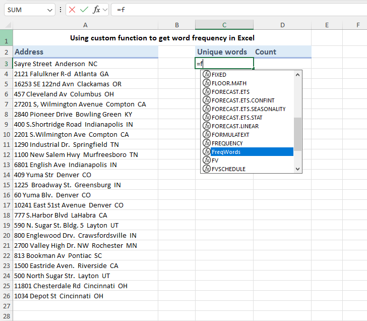
Tip. Unfortunately, Excel doesn't display tooltips for custom function arguments like it does for built-in functions. However, there's a little trick to display argument names. Simply enter the name of the custom function and then press the Ctrl + Shift + A shortcut. For more details, see how to display tooltips for custom VBA functions in Excel.
Alternatively, you can use the Function Wizard to configure the FreqWords function, as explained in the tutorial linked above.
Using FreqWords function in Excel 365 and 2021
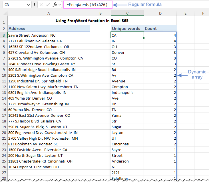
In Dynamic Array Excel, FreqWord behaves like a dynamic array function, i.e. you enter a formula in one cell and it returns an array of values into neighboring cells.
Using FreqWords function in Excel 2019 - 2007
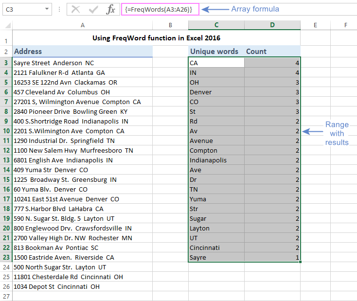
In pre-dynamic versions of Excel, you need to use the FreqWords function as an array formula, which requires a slightly different approach:
- Select the destination range. Select a range of empty cells where you want the results to appear. These cells will be populated with the word frequencies.
- Enter the formula. Type the FreqWords formula in the formula bar.
- Make it an array formula. Here's the crucial step - instead of just pressing Enter, press the Ctrl + Shift + Enter key combination. This tells Excel to treat the formula as an array formula and calculate it accordingly.
For more information, see How to enter an array formula in Excel.
Now that you understand how to use the FreqWords function, let's look at some real-life scenarios where it can simplify your Excel data work.
How to count frequency of words in Excel
Let's assume you have a list of addresses in A2:A25. To find out which words most often occur in this list, enter this formula in C3:
=FreqWords(A2:A25)
After hitting Enter, you will receive a list of all unique words and the number of times each word appears in the source range. The words will be displayed in column C, and their corresponding frequencies will be in column D.
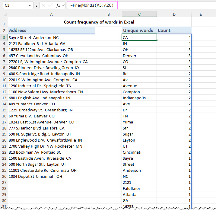
In Excel 365 and Excel 2021, the formula returns an array of values in multiple cells. However, in Excel 2019 and earlier versions, a normal formula will return just a single value. To obtain a list of values, be sure to enter it as an array formula as explained above.
How to do word frequency analysis with custom delimiter
Often, when importing data into Excel from other programs or CSV files, values are not separated by spaces but by special characters such as commas, semicolons, colons, slashes, and more.
In such cases, you need to specify the second argument [delimiter] of the FreqWords function.
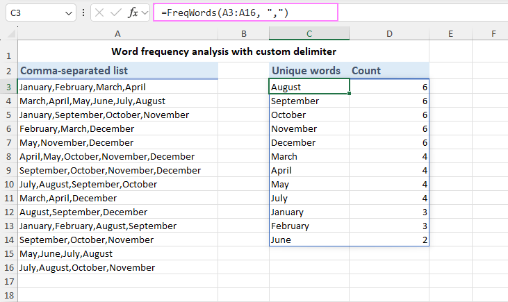
For example, to calculate the frequency of words in a comma-separated list in A3:A16, use the following formula:
=FreqWords(A3:A16, ",")
If your values are separated by another character, replace "," with your specific delimiter as needed.
The result of this calculation is a frequency table of words based on your specified delimiter:
How to count frequency of text within one cell
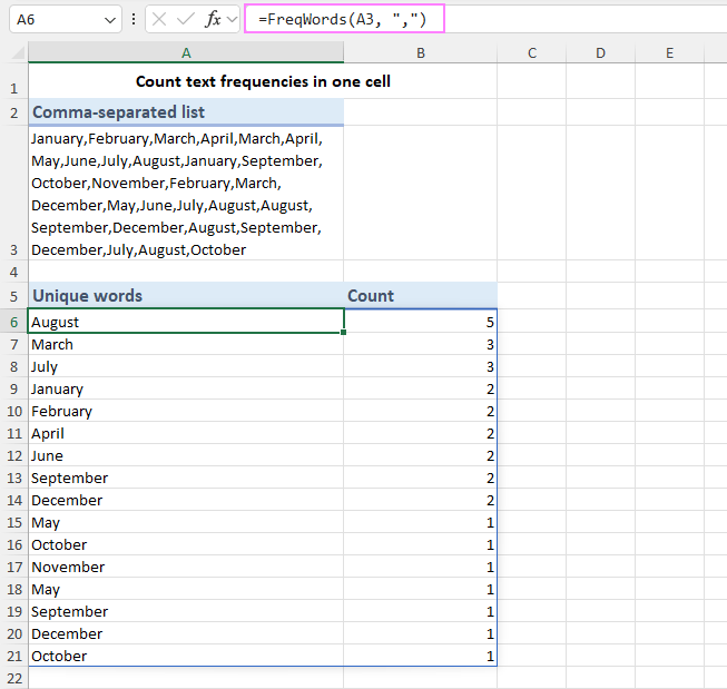
In case you need to count text frequencies within a single cell, simply supply that cell address for the first argument of the FreqWords function:
=FreqWords(A3, ",")
As a result, you’ll get the following word frequency list:
How to compare frequency of words in two columns
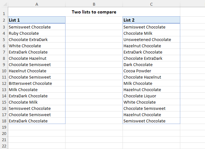
Microsoft Excel offers various methods to compare columns and identify duplicate and unique values in two lists. However, there are situations where you need to compare not the entire cell values, but the frequencies of words within each column, regardless of their position or order in the cells. This is where the FreqWords function becomes invaluable!
Let's consider a scenario where you have two lists with similar items but in different orders. Moreover, the items in these lists may have different word arrangements, such as "chocolate milk" and "milk chocolate". The question is: are these lists identical or different?
The solution involves two simple steps.
Step 1: Find frequency of words in each list
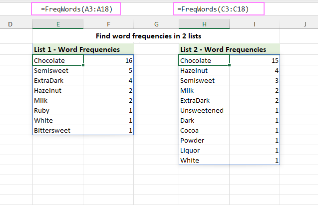
To determine how many times each word appears in each list, use the FreqWords function in its basic form.
Word frequencies in List 1:
=FreqWords(A3:A18)
Word frequencies in List 2:
=FreqWords(C3:C18)
By applying these formulas, you obtain the word count for each list. Examining the results, as shown in the screenshot below, you can conclusively determine that the two lists are different.
Step 2: Compare word frequencies in two lists
Once you've established that the compared lists are different, you may want to delve deeper and gather more details, such as:
- Which words appear in both lists, and which are unique to one list?
- Which words have the same number of occurrences in both lists, and which occur a different number of times?
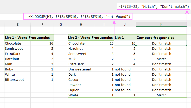
To accomplish this task, you need to place the word frequencies side by side. In our example, since List 2 contains more unique words, we'll consider it the main list and pull the frequencies from List 1 to the adjacent column using the XLOOKUP function.
The formula below goes to cell J3, and then you copy it down the column:
=XLOOKUP(H3, $E$3:$E$10, $F$3:$F$10, "not found")
By comparing the word counts in columns I (List 1) and J (List 2), you can clearly see how many times each word occurs in both lists. And the “not found” text in column J indicates that a word is not present in List 2.
To make the differences even more apparent, you can add labels such as "match" and "don't match" in a separate column. This can be achieved using the following IF statement that compares the word counts in columns I and J:
=IF(I3=J3, "Match", "Don’t match")
“Match” means a given word has the same number of occurrences in both lists. “Don’t match” means a word occurs only in one list or has a different number of occurrences.
This is an effective approach when dealing with text data that have words in a different order or mixtures. It also works great for comparing text frequencies in two lists with many words in each cell, separated by any character. Plus, it's handy for comparing really big cells, even the extra-large ones containing dozens or hundreds of different words.
Highlight matches and differences in word frequency tables
Using the formulas discussed above, you can effectively compare text frequencies in two columns. To gain even more valuable insights into the similarities and differences between two lists, you can highlight these distinctions with colors. This can be easily accomplished with the Compare Tables tool, a part of our Ultimate Suite for Excel.
As an example, let's compare the word frequency lists obtained by applying the FreqWords function: Table 1 (A3:B10) and Table 2 (D3:E13).
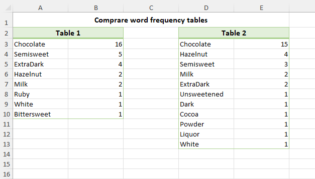
You can find detailed guidance on using the Compare Tables tool in the online documentation. Here, we'll provide a brief overview of the steps:
- Select the first table (A3:B10).
- Select the second table for comparison (D3:E13).
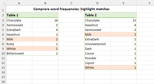
- Specify whether you want to find Duplicates (items that occur in both lists) or Unique Values (differences between the two lists). We opt for duplicates, i.e. finding the same word counts in both tables.
- Select the columns for comparison. This is the key step, so carefully make your selections. In this example, we choose two column pairs, which include words and their respective frequencies.

- Finally, select the action you want to take – for example, highlighting with a specific color. Then, click the Finish button.
- Repeat the same steps to compare Table 2 to Table 1.
As a result, you'll get the same word frequencies highlighted in both lists, allowing you to visually distinguish matches and differences.
To wrap it up, analyzing text frequencies in Excel doesn't have to be tough anymore. With the custom FreqWords function and the Compare Tables tool, it becomes super simple! Whether you're working on textual analysis, data mining, or simply trying to figure out the patterns in your spreadsheet, these tools together will make your tasks smoother and more understandable. Just give them a try and see the difference they can make.
If you still have any questions or want to share your thoughts on this topic, feel free to drop a few lines in the Comments down below :)
Available downloads
Count words frequencies – formula examples (.xlsm file)
Ultimate Suite 14-day fully-functional version (.exe file)
 by
by